|
|
Pubmedy:显示影响因子+引用数、Sci-hub全文下载的浏览器扩展
很多人都知道一个下载文献的好地方 Sci-Hub,但是现在 Sci-Hub 的站长 Alexandra Elbakyan 女士面临着爱思唯尔的诉讼,让其面临数百万美元的赔偿。因此现在 Sci-Hub 在某些时候可能不可用了。不过 Alexandra Elbakyan 女士并未妥协,希望大家能多支持一下这位女士(貌似只能接受比特币捐款,我也不知道怎么弄,要是paypal或者payoneer就好了)。
相信很多人都知道下面这两个网址:
Sci-Hub 官网:http://www.sci-hub.org/
Sci-Hub 替代网址:http://www.sci-hub.io/
http://sci-hub.ac/和http://sci-hub.cc/也都已经阵亡(2017月12月6日测试)
以上几个网址都挂了,现在可用的是
http://sci-hub.bz/(12月8日测试 已经不可用了)
http://sci-hub.la/
http://sci-hub.hk/
http://sci-hub.tw/
http://sci-hub.tv/
http://80.82.77.83/
http://80.82.77.84/
Workspace loaded from ~/.RData]

> setwd("/home/shenzy/work/beast/51samples")
> library(seqinr)
> data=read.fasta("51strain_core_gene_alignment.aln")
> library(ape)

Attaching package: ‘ape’

The following objects are masked from ‘package:seqinr’:

    as.alignment, consensus

> write.nexus.data(data,file="51strain_core_gene_alignment.aln.nexus", format="DNA")
|
|
|
|
axes : matplotlib/pylab axes If a valid matplotlib.axes.Axes instance, the phylogram is plotted in that Axes. By default (None), a new figure is created.
This means that you can load your own axes with your size of choice. For example
import matplotlib
import matplotlib.pyplot as plt
from Bio import Phylo
from cStringIO import StringIO

def plot_tree(treedata, output_file):
    handle = StringIO(treedata)  # parse the newick string
    tree = Phylo.read(handle, "newick")
    matplotlib.rc('font', size=6)
    # set the size of the figure
    fig = plt.figure(figsize=(10, 20), dpi=100)
    # alternatively
    # fig.set_size_inches(10, 20)
    axes = fig.add_subplot(1, 1, 1)
    Phylo.draw(tree, axes=axes)
    plt.savefig(output_file, dpi=100)

    return


#!/usr/bin/env python

from Bio import Phylo
from cStringIO import StringIO
from matplotlib import pyplot as plt
import csv
import argparse
import os
import matplotlib


import matplotlib.font_manager as font_manager

colors = dict(Expansions='green', Contractions='red', Rapid='blue')

labels = dict()

def display(tree_type):
 if tree_type == 'Rapid':
 return 'Rapidly evolving families'

 else:
 return tree_type


def label(n):
 family_count = n.info
 if n.name:
 return "%s (%s)" % (n.name, family_count)

 else:
 return family_count

def prettify_tree(fig):
 plt.ylabel('')


 plt.tick_params(
 axis='y', # changes apply to the y-axis
 which='both', # both major and minor ticks are affected
 left='off', # ticks along the left edge are off
 right='off', # ticks along the right edge are off
 labelleft='off') # labels along the left edge are off

 [fig.gca().spines[border].set_visible(False) for border in ['left', 'right', 'top']]

def draw_tree(datafile, tree_type, newick, node_ids, output_file):
 with open(datafile) as f:
 reader = csv.DictReader(f, delimiter='\t')

 for row in reader:
 labels[row["Node"]] = row

 tree = Phylo.read(StringIO(newick), "newick")
 id_tree = Phylo.read(StringIO(node_ids), "newick")

 for clade, c_id in zip(tree.find_clades(), id_tree.find_clades()):
 clade.info = labels[c_id.name][display(tree_type)] if c_id.name in labels else ""

 tree.ladderize() # Flip branches so deeper clades are displayed at top


 plt.ion()
 fig = plt.figure(frameon=False)
 matplotlib.rc('font', size=6)

 Phylo.draw(tree, axes=fig.gca(), do_show=False, label_func=label, label_colors = lambda n: colors[tree_type])
 plt.title(display(tree_type) + " (count)")
 prettify_tree(fig)
 plt.ioff()

 if output_file:
 fig.savefig(output_file, format='png', bbox_inches='tight', pad_inches=0, dpi=180)

 else:
 plt.show()


if __name__ == "__main__":
 parser = argparse.ArgumentParser(description=__doc__, prog="draw_expansion_tree.py")
 parser.add_argument("-i", "--input-file", action="store", dest="input_file", required=True, type=str, help="full path to mcl's output dump file")
 parser.add_argument("-t", "--tree", action="store", dest="tree", required=True, help="Newick tree to display")
 parser.add_argument("-d", "--ids", action="store", dest="id_tree", required=True, help="Matching Newick tree with node IDs")
 parser.add_argument("-y", "--tree-type", action="store", dest="tree_type", default="Expansions", required=False, type=str, help="Expansions, Contractions, or Rapid")
 parser.add_argument("-o", "--output-file", action="store", dest="output_file", required=False, type=str, help="output PNG file name")

 args = parser.parse_args()

 if not os.path.isfile(args.input_file):
 exit("Could not find input file. Exiting...\n")

 draw_tree(args.input_file, args.tree_type, args.tree, args.id_tree, args.output_file)
One of the common problem while working in UNIX is to find large files to free some space. Suppose, your file system is full and you are receiving an alert to remove spaces or if your host is run out of space and your server is not starting up, the first thing you do is find top 10 largest files and see if you can delete them. Usually, old files, large Java heap dumb are good candidates for removal and freeing up some space. If you are running Java application e.g. core java based programs or web application running on Tomcat then you can remove those heap dump files and free some space, but the big question is how do you find those? How do you know the size of the biggest file in your file system, especially if you don’t know which directory it is? We’ll try to find answers for some of those questions in this article.
When I was new to Linux, I don’t have any other choice but to go to the log directory and look for old files which are larger among rest and delete them. They worked well until one day our server died due to a huge cache file. I wasn’t able to locate that because it wasn’t in the log directory, then I come to know about find command which let you search sub-directories for large files as shown below:
$ find . -size +1G
This command will print all the files which are greater than 1GB from current directory and any subdirectory. The only problem with this one is that it doesn’t print the exact size. The problem was solved by using the -printf option, which allows you to specify a format String much like Java’s printf() method. See Linux Command Line Interface (CLI) Fundamentals to learn more about various options of find command in Linux.
You can further tweak the command to find files up-to certain size e.g. below command will find all files. Here is the modified UNIX command to find large files with size :
$ find . -size +1G -printf ‘%s %p\n’
here is %s is for size and %p are for the path.
Alternatively, You can also use -exec option to run ls on each file the find command return to print its size as shown below:
$ find . -size +100M -exec ls -sh {} \;
This is good enough, you can just see which files you can delete and free some space, but problem is that you will not find any file which is larger than 1GB, hence I always use this command with some hypothetical large number e.g. 10GB etc, but, those are just workaround, not the proper fix. Let’s see what we can do next.
Btw, you can also use the du (disk usage) command to find large directories and their size, as shown below :
$ du -a . | sort -n -r | head -n 10
16095096 .
13785288 ./logs
6095380 ./logs/app
2125252 ./temp
2125244 ./temp/data
2125240 ./temp/data/app
This is the right command, it will list both directories and file. I have also combined the output of the du command with sort command to print the top 10 largest file and directories. This is exactly what we are looking for. In fact, this is also one of the frequently asked Linux Interview questions, so if you know this trick you answer this question on interviews as well.
That’s all about how to find the large files and directories in Linux. As I said, earlier I used to search large files by using find command with -size option but that is more or less a guess work because you never know the size of the largest file in a machine, but by using a reasonable high size, you can possibly find all big files in your filesystem. One more command you can use to find the large files with size in Linux is the disk usage or du command, which will also list both files and directories.
熟悉我们生信技能树团队的应该都知道大名鼎鼎的y叔啦,作为我们论坛的荣誉顾问,y叔一直勤勤恳恳的指出我们的错误,特意在此谢谢y叔!并奉上y叔的ChIP-seq数据分析大礼包,已经征得y叔同意啦!
关注Y叔微信公众账号biobabble

接下来要出一个ChIPseq系列,讲一讲ChIPseq和我的ChIPseeker包,从入门到放弃是我自己的个人写照。我做ChIPseq总共也就3个月的时间,做的事情并不多,在一知半解的情况下写下了ChIPseeker包。
正如我在《话题投票》里说的,我当时被要求做ChIPseq分析是为他人做嫁衣,而且是完全白干那种,但做为学生,白干也得干。

当时一开始使用ChIPpeakAnno做注释,但用UCSC genome browser检验结果的时候,发现对不上。在对ChIPpeakAnno包不满意的情况下,开始着手写ChIPseeker,其实在使用ChIPpeakAnno的时候,我就有写代码对结果做一些可视化,所以未有ChIPseeker先有ChIPseeker的部分可视化功能。当时写了篇博客文说ChIPpeakAnno的问题,一个月后就在Bioconductor上发表了ChIPseeker,这包完全是我半夜在宿舍里写出来的。
当时还在生物系,被我炒掉的前老板每天要求必须起码在实验室待够12小时,我每天都待到10点半左右才回宿舍,日常在实验室里啥都干不了,白天各种瞎折腾,晚上还要陪他聊天,但说来说去,每天几乎都差不多,无非是他很牛逼,我们这帮人读他phd实在太幸运,日复一日传销式洗脑。而我因为结婚了,家又离得近,周末回家,白天经常多一段单独对我的洗脑,做为一个PhD学生,在发表文章之前是不能够有周末的。每天10半从实验室里出来,回到宿舍11点,跟老婆打电话再洗澡,12点。然后从12点开始写代码到2点睡觉,才有了这个包。
虽然是一知半解的时候开发的,但还是受到大家的欢迎,半年前Matt邀请我去人大做报告时,也专门提到了ChIPseeker。

也有美国的助理教授,跟我要paper,说是上课的时候,要给学生读的,这广告效果我给满分。

文章发表了一年,已经被33篇文章引用,其中不乏有影响因子比较高的杂志:

下面是其中一些引用文章的图:


虽然ChIPseeker是我写给自己做ChIPseq注释的,但Ming Tang (https://github.com/crazyhottommy/ChIP-seq-analysis)用它去做DNA breakdown注释,当然像lincRNA注释也是有人做并且完全是支持的。有一些我以前从没在文档里提到的东西,也应该会在这个系列里写出来。
这个系列基本上是围绕着ChIPseeker的功能而来,名副其实从入门到放弃,因为我自己也是入了门然后放弃,如果想看从入门到精通的,这显然不适合你。
然而今天只是个剧透,敬请期待。
ChIP是指染色质免疫沉淀,它通特异结合抗体将DNA结合蛋白免疫沉淀,可以用于捕获蛋白质(如转录因子,组蛋白修饰)的DNA靶点。这技术存在非常久了,在二代测序之前,结合microarray,它的名字叫ChIP-on-chip,二代测序出来之后,显而易见的,免疫沉淀拉下来的DNA拿去NGS测序,这必然是下一代的ChIP技术,优点也是显而易见的,不再需要设计探针(往往存在着一定的偏向性)。所以NGS出来以后,不差钱的牛逼实验室显然占据上风,谁先做出来,谁就定义了新技术。这是有钱人的竞赛,没钱的只能等着技术烂大街的时候跟风做。
这是显而易见的下一代技术,外加技术上完全是可行的,所以这是一场单纯的时间竞赛,于是几乎同时出来CNS文章,基本上谁也不比谁差地同时扔出来。
- Johnson DS, Mortazavi A et al. (2007) Genome-wide mapping of in vivo protein–DNA interactions. Science 316: 1497–1502
- Robertson G et al.(2007) Genome-wide profiles of STAT1 DNA association using chromatin immunoprecipitation and massively parallel sequencing. Nature Methods 4: 651–657
- Schmid et al. (2007) ChIP-Seq Data reveal nucleosome architecture of human promoters. Cell 131: 831–832
2007年来自三个不同的实验室,几乎是同时间出来(最长差不了3个月),分别发CNS,一起定义了这个ChIPseq技术。

这个技术分为4步:
- Cross-linking
- Sonication
- IP
- Sequencing
DNA和蛋白质交联(cross-linking),超声(sonication)将染色体随机切割,利用抗原抗体的特异性识别(IP),把目标蛋白相结合的DNA片段沉淀下来,反交联释放DNA片段,最后是测序(sequencing)。
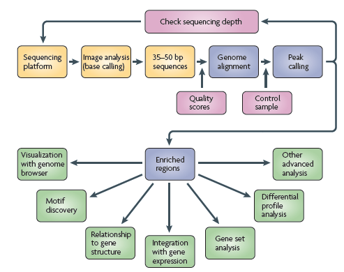
一个典型的分析流程如下:

测序之后,我们当然首先需要做质量控制,然后就是做mapping,拿到这些DNA片段在染色体上的位置信息,ChIPseq的数据我们还需要做peak calling,把背景噪声去掉,比如上图中使用MACS做peak calling,这样我们就得到了protein binding site (peak),就可以做下游的分析,比如可视化、相关的基因(比如最近的基因、宿主基因)、Motif分析等等。
Peak annotation做的就是binding site的相关基因注释,在讲解ChIPseeker的注释功能之前,下次先讲解一下peak calling的输出,BED文件。
文件格式
BED的全称是Browser Extensible Data,顾名思义是为genome browser设计的,大名鼎鼎的bedtools可不是什么「床上用品」。
BED包含有3个必须的字段和9个可选字段。
三个字段包括:
- 1 chrom – 染色体名字
- 2 chromStart – 染色体起始位点
- 3 chromEnd – 染色体终止位点
这里必须指出的是chromStart是起始于0,而不是1。很多分析软件都忽略了这一点,会有一个碱基的位移,据我说知Homer和ChIPseeker没有这个问题,而像peakAnalyzer, ChIPpeakAnno等都有位移的问题。
可选的9个字段包括:
- 4 name – 名字
- 5 score – 分值(0-1000), 用于genome browser展示时上色。
- 6 strand – 正负链,对于ChIPseq数据来说,一般没有正负链信息。
- 7 thickStart – 画矩形的起点
- 8 thickEnd – 画矩形的终点
- 9 itemRgb – RGB值
- 10 blockCount – 子元件(比如外显子)的数目
- 11 blockSizes – 子元件的大小
- 12 blockStarts – 子元件的起始位点
一般情况下,我们只用到前面5个字段,这也是做peak calling的MACS输出的字段。
其中第5个字段,MACS的解释是这样子的:
The 5th column in this file is the summit height of fragment pileup.
是片段堆积的峰高,这也不难理解,为什么我在ChIPseeker是画peak coverage的函数covplot要有个weightCol的参数了。
数据可视化
从名字上看,它是为genome browser而生,相应的,ChIPseeker实现了covplot来可视化BED数据。
covplot支持直接读文件出图:
library(ChIPseeker)
library(ggplot2)

files <- getSampleFiles()
covplot(files[[4]])

支持GRanges对象,同时可以多个文件或者GRangesList
peak=GenomicRanges::GRangesList(CBX6=readPeakFile(files[[4]]),CBX7=readPeakFile(files[[5]]))
covplot(peak, weightCol="V5") + facet_grid(chr ~ .id)

支持可视化某个窗口
covplot(peak, weightCol="V5", chrs=c("chr17", "chr18"), xlim=c(4e7, 5e7)) + facet_grid(chr ~ .id)

拿到数据后,我们首先会可视化看一下数据,接下来就会想知道这些peak都和什么样的基因有关,这将在下次讲解,如何做注释。(昨天biostars上就有人在问用ChIPseeker给schizosaccharomyces pombe裂殖酵母做注释,大家可去围观)
这一次讲解非常重要的peak注释,注释在ChIPseeker里只需要用到一个函数annotatePeak,它可以满足大家各方面的需求。
输入
当然需要我们上次讲到的BED文件,ChIPseeker自带了5个BED文件,用getSampleFiles()可以拿到文件的全路径,它返回的是个named list,我这里取第4个文件来演示。annotatePeak的输入也可以是GRanges对象,你如果用R做peak calling的话,直接就可以衔接上ChIPseeker了。
> require(ChIPseeker)
> f = getSampleFiles()[[4]]
巧妇难为无米之炊,就像拿到fastq要跑BWA,你需要全基因组的序列一样,做注释当然需要注释信息,基因的起始终止,基因有那些内含子,外显子,以及它们的起始终止,非编码区的位置,功能元件的位置等各种信息。
很多软件会针对特定的物种去整理这些信息供软件使用,但这样就限制了软件的物种支持,有些开发者写软件本意也是解决自己的问题,可能对自己的研究无关的物种也没兴趣去支持。
然而ChIPseeker支持所有的物种,你没有看错,ChIPseeker没有物种限制,当然这是有前提的,物种本身起码是有基因的位置这些注释信息,不然就变无米之炊了。
这里我们需要的是一个TxDb对象,这个TxDb就包含了我们需要的各种信息,ChIPseeker会把信息抽取出来,用于注释时使用。
> require(TxDb.Hsapiens.UCSC.hg19.knownGene)
> txdb = TxDb.Hsapiens.UCSC.hg19.knownGene
> x = annotatePeak(f, tssRegion=c(-1000, 1000), TxDb=txdb)
>> loading peak file...                 2017-03-09 11:29:18 PM
>> preparing features information...         2017-03-09 11:29:18 PM
>> identifying nearest features...         2017-03-09 11:29:19 PM
>> calculating distance from peak to TSS...     2017-03-09 11:29:20 PM
>> assigning genomic annotation...         2017-03-09 11:29:20 PM
>> assigning chromosome lengths             2017-03-09 11:29:42 PM
>> done...                     2017-03-09 11:29:42 PM
这里需要注意的是,启动子区域是没有明确的定义的,所以你可能需要指定tssRegion,把基因起始转录位点的上下游区域来做为启动子区域。
有了这两个输入(BED文件和TxDb对象),你就可以跑注释了,然后就可以出结果了。
输出
如果在R里打输出的对象,它会告诉我们ChIPseq的位点落在基因组上什么样的区域,分布情况如何。
> x
Annotated peaks generated by ChIPseeker
1331/1331  peaks were annotated
Genomic Annotation Summary:
             Feature  Frequency
9           Promoter 48.1592787
4             5' UTR  0.7513148
3             3' UTR  4.2073629
1           1st Exon  0.7513148
7         Other Exon  3.9068370
2         1st Intron  3.6814425
8       Other Intron  7.7385424
6 Downstream (<=3kb)  1.1269722
5  Distal Intergenic 29.6769346
如果我想看具体的信息呢?你可以用as.GRanges方法,这里我只打印前三行:

Bioconductor里有很多包是针对GRanges对象的,这样方便你在R里做后续的处理,如果你说你不懂这些,只想输出个Excel表格。那么也很容易,用as.data.frame就可以转成data.frame,然后你就可以用write.table输出表格了。
两种不同的注释
这里注释有两种,一种是genomic annotation (也就是annotation这一列)还有就是nearest gene annotation(也就是多出来的其它列)。
经常有人问我问题,把这两种搞混。genomic annotation注释的是peak的位置,它落在什么地方了,可以是UTR,可以是内含子或者外显子。
而最近基因是peak相对于转录起始位点的距离,不管这个peak是落在内含子或者别的什么位置上,即使它落在基因间区上,我都能够找到一个离它最近的基因(即使它可能非常远)。
这两种注释的策略是不一样的。针对不同的问题。第一种策略peak所在位置,可能就是调控的根本,比如你要做可变剪切的,最近基因的注释显然不是你关注的点。
而做基因表达调控的,当然promoter区域是重点,离结合位点最近的基因更有可能被调控。
最近基因的注释信息虽然是以基因为单位给出,但我们针对的是转录起始位点来计算距离,针对于不同的转录本,一个基因可能有多个转录起始位点,所以注释是在转录本的水平上进行的,我们可以看到输出有一列是transcriptId.
第三种注释
两种注释有时候还不够,我想看peak上下游某个范围内(比如说-5k到5k的距离)都有什么基因,annotatePeak也可以做到。
你只要传个参数说你要这个信息,还有什么区间内,就可以了。
x = annotatePeak(f[[4]], tssRegion=c(-1000, 1000), TxDb=txdb, addFlankGeneInfo=TRUE, flankDistance=5000)

输出中多三列: flank_txIds, flank_geneIds和flank_gene_distances,在指定范围内所有的基因都被列出。
基因注释
对于通常情况找最近基因的策略,最近基因给出来了,但都是各种人类不友好的ID,我们不能把一切都交给计算机,输出的结果我们还是要看一看的,能不能把基因的ID换成对人类友好的基因名,并给出描述性的全称,这个必然可以有。
只需要给annotatePeak传入annoDb参数就行了。
如果你的TxDb的基因ID是Entrez,它会转成ENSEMBL,反之亦然,当然不管是那一种,都会给出SYMBOL,还有描述性的GENENAME.
为什么我要用某个基因组版本?
在上一篇文章中,我用了TxDb.Hsapiens.UCSC.hg19.knownGene。 hg19的TxDb, 或者有人就要问了,为什么不用hg38?
这个问题,不是说要用那一个,不能用那一个。而是你必须得用某一个,这取决于你最初fastq用BWA/Bowtie2比对于某个版本的基因组,你最初用了某个版本,后面就得用相应的版本,不能混,因为不同版本的位置信息有所不同。
当然如果要(贵圈喜欢的)强搞,也不是不可以,你得有chain file,先跑个liftOver,实际上就是在两个基因组版本之间做了位置转换。
为什么说ChIPseeker支持所有物种?
背景注释信息用了TxDb就能保证所有物种都支持了?我去哪里找我要的TxDb?
我写ChIPseeker的时候,我做的物种是人,ChIPseeker在线一周就有剑桥大学的人写信跟我说在用ChIPseeker做果蝇,在《CS2: BED文件》一文中,也提到了最近有人在Biostars上问用ChIPseeker做裂殖酵母。
首先Bioconductor提供了30个TxDb包,可以供我们使用,这当然只能覆盖到一小部分物种,我们的物种基因组信息,多半要从UCSC或者Ensembl获得,我敢说支持所有物种,就是因为UCSC和ensembl上所有的基因组都可以被ChIPseeker支持。
因为我们可以使用GenomicFeatures包函数来制作TxDb对象:
- makeTxDbFromUCSC: 通过UCSC在线制作TxDb
- makeTxDbFromBiomart: 通过ensembl在线制作TxDb
- makeTxDbFromGRanges:通过GRanges对象制作TxDb
- makeTxDbFromGFF:通过解析GFF文件制作TxDb
比如我想用人的参考基因信息来做注释,我们可以直接在线从UCSC生成TxDb:
require(GenomicFeatures)
hg19.refseq.db <- makeTxDbFromUCSC(genome="hg19", table="refGene")
比如最近在biostars上有用户问到的,做裂殖酵母的注释,我们可以下载相应的GFF文件,然后通过makeTxDbFromGFF函数生成TxDb对象,像下面的命令所演示,spombe就是生成的TxDb,就可以拿来做裂殖酵母的ChIPseq注释。
download.file("ftp://ftp.ebi.ac.uk/pub/databases/pombase/pombe/Chromosome_Dumps/gff3/schizosaccharomyces_pombe.chr.gff3", "schizosaccharomyces_pombe.chr.gff3")require(GenomicFeatures)
spombe <- makeTxDbFromGFF("schizosaccharomyces_pombe.chr.gff3")
所以我敢说,所有物种都支持。像Johns Hopkins出品的CisGenome就只支持到12个物种而已,极大地限制了它的应用。
ChIPseeker有什么不能注释的吗?
这个我还没想到,像CpG是不支持的,但也有人「黑」出来了:

当然他的做法是把CpG也整合进去,如果你单纯只想看那些peak落在CpG上,或者说离CpG最近,不需要「黑」也能做到的,因为annotatePeak的背景注释信息除了TxDb之外,其实它还可以是自定义的GRanges对象,这保证了用户各种各样的需求,因为TxDb也不是万能的,如果能自定义,比如说我就只想看蛋白的结合位点会不会在内含子和外显子的交界处,再比如说我做的并不是编码蛋白的基因表达调控,而是非编码RNA,那么我想要用lncRNA的位置信息来做注释。像这样的需求,ChIPseeker都是可以满足的。
可以按正负链分开注释吗?
上一篇文章《CS3: peak注释》中就有人问了,能否同时给出正负链上最近的基因。首先ChIPseq数据通常情况下是没有正负链信息的(有特殊的实验可以有),annotatePeak函数有参数是sameStrand,默认是FALSE,你可以给你的peak分别赋正负链,然后传入sameStrand=TRUE,分开做两次,你就可以分开拿到正链和负链的最近基因。
最近基因位置是相对于TSS的,能否相对于整个基因?
答案也是可以的!
首先如果peak和TSS有overlap,genomic annotation就是promoter,而最近基因也是同一个,所以在这种情况下,两种注释都指向同一个基因,可以说信息是冗余的,能不能不要冗余信息?这个是可以的,你可以传入参数ignoreOverlap=TRUE,那么最近基因就会去找不overlap的。
最近基因是相对于TSS,如果和TSS有overlap,距离是0, 必须是最近。回到标题的问题,如果我想说只要和基因有overlap就是最近基因,这种情况其实你的最近基因就是host gene,也就是annotation这个column给出来的是相对应的,我们就想找peak所在位置的基因信息,那么这当然也是可以的,默认参数overlap=”TSS”, 如果改为overlap=”all”,它看的就是整个基因而不是TSS,当然distanceToTSS也还是会计算,如果overlap的不是TSS,而是基因体里,并不会因为而设为0。
如果我只想注释上游或者是下游的基因呢?
当然也可以,我们有ignoreUpstream和ignoreDownstream参数,默认都是FALSE。随便你想看上游还是下游,都可以。
为什么要有这么多参数?
我在前一篇,只讲了输入,输出,你知道两个输入,会看输出,你就可以做ChIPseq注释了,非常简单。但是我不能把annotatePeak能做的全列出来,会让大家觉得复杂。(而且简单的情况是最常见的行为)
在大家知道输入输出,觉得简单之后,再讲一讲,它有一些参数,可以应对别的情况,这些情况可能并不是我们做ChIPseq所需要的,但不同参数的灵活组合,是可以解决和应对不同的需求的。
比如说, DNA是可以断的,如果我们要对(DNA breakpoints)断点位置做注释,优先是overlap基因,再者是上游,你会发现很多软件都不能做了,但ChIPseeker可以。
https://guangchuangyu.github.io/2014/04/chipseeker-for-chip-peak-annotation/
ChIPpeakAnno WAS the only R package for ChIP peak annotation. I used it for annotating peak in my recent study.
I found it does not consider the strand information of genes. I reported the bug to the authors, but they are reluctant to change.
So I decided to develop my own package, ChIPseeker, and it’s now available in Bioconductor.
> require(TxDb.Hsapiens.UCSC.hg19.knownGene)
> txdb <- TxDb.Hsapiens.UCSC.hg19.knownGene
> require(ChIPseeker)
> peakfile = getSampleFiles()[[4]]
> peakfile
[1] "/usr/local/Cellar/r/3.1.0/R.framework/Versions/3.1/Resources/library/ChIPseeker/extdata//GEO_sample_data/GSM1295076_CBX6_BF_ChipSeq_mergedReps_peaks.bed.gz"
> peakAnno <- annotatePeak(peakfile, tssRegion=c(-3000, 1000), TxDb=txdb, annoDb="org.Hs.eg.db")
>> loading peak file...              2014-04-13 12:03:45 PM
>> preparing features information...         2014-04-13 12:03:45 PM
>> identifying nearest features...       2014-04-13 12:03:45 PM
>> calculating distance from peak to TSS...  2014-04-13 12:03:46 PM
>> assigning genomic annotation...       2014-04-13 12:03:46 PM
>> adding gene annotation...             2014-04-13 12:03:50 PM
>> assigning chromosome lengths          2014-04-13 12:03:50 PM
>> done...                   2014-04-13 12:03:50 PM
> head(as.GRanges(peakAnno))
GRanges object with 6 ranges and 14 metadata columns:
      seqnames             ranges strand |          V4        V5
                      |
  [1]     chr1 [ 815092,  817883]      * | MACS_peak_1    295.76
  [2]     chr1 [1243287, 1244338]      * | MACS_peak_2     63.19
  [3]     chr1 [2979976, 2981228]      * | MACS_peak_3    100.16
  [4]     chr1 [3566181, 3567876]      * | MACS_peak_4    558.89
  [5]     chr1 [3816545, 3818111]      * | MACS_peak_5     57.57
  [6]     chr1 [6304864, 6305704]      * | MACS_peak_6     54.57
             annotation  geneChr geneStart   geneEnd geneLength geneStrand

  [1] Distal Intergenic     chr1    803451    812182       8732          -
  [2]  Promoter (<=1kb)     chr1   1243994   1247057       3064          +
  [3]  Promoter (<=1kb)     chr1   2976181   2980350       4170          -
  [4]  Promoter (<=1kb)     chr1   3547331   3566671      19341          -
  [5]  Promoter (<=1kb)     chr1   3816968   3832011      15044          +
  [6]            3  UTR     chr1   6304252   6305638       1387          +
           geneId transcriptId distanceToTSS         ENSEMBL      SYMBOL

  [1]      284593   uc001abt.4         -5701 ENSG00000230368      FAM41C
  [2]      126789   uc001aed.3             0 ENSG00000169972       PUSL1
  [3]      440556   uc001aka.3             0 ENSG00000177133   LINC00982
  [4]       49856   uc001ako.3             0 ENSG00000116213      WRAP73
  [5]   100133612   uc001alg.3             0 ENSG00000236423   LINC01134
  [6]      390992   uc009vly.2          1452 ENSG00000173673        HES3
                                          GENENAME

  [1] family with sequence similarity 41, member C
  [2]              pseudouridylate synthase-like 1
  [3]   long intergenic non-protein coding RNA 982
  [4]      WD repeat containing, antisense to TP73
  [5]  long intergenic non-protein coding RNA 1134
  [6]       hes family bHLH transcription factor 3
  ---
  seqlengths:
        chr1     chr10     chr11     chr12 ...      chr8      chr9      chrX
   249250621 135534747 135006516 133851895 ... 146364022 141213431 155270560
annotatePeak function can accept peak file or GRanges object that contained peak information. The sample peakfile shown above is a sample output from MACS. All the information contained in peakfile will be kept in the output of annotatePeak.
The annotation column annotates genomic features of the peak, that is whether peak is located in Promoter, Exon, UTR, Intron or Intergenic. If the peak is annotated by Exon or Intron, more detail information will be provided. For instance, Exon (38885 exon 3 of 11) indicates that the peak is located at the 3th exon of gene 38885 (entrezgene ID) which contain 11 exons in total.
All the names of column that contains information of nearest gene annotated will start with gene in camelCaps style.
If parameter annoDb=“org.Hs.eg.db” is provided, extra columns of ENSEMBL, SYMBOL and GENENAME will be provided in the final output.
For more detail, please refer to the package vignette. Comments or suggestions are welcome.
——- below was added at April 30, 2014 ———–
After two weeks of ChIPseeker release in Bioconductor, I am very glad to receive an email from Cambridge Systems Biology Centre that they are using ChIPseeker in annotating Drosophila ChIP data.
Although I only illustrate examples in human, ChIPseeker do supports all species only if genomic information was available. 
> require(TxDb.Dmelanogaster.UCSC.dm3.ensGene)
> require(ChIPseeker)
> txdb <- TxDb.Dmelanogaster.UCSC.dm3.ensGene
>
> chr <- c("chrX", "chrX", "chrX")
> start <- c(71349, 77124, 86364)
> end <- c(72835, 77836, 88378)
> peak <- GRanges(seqnames = chr, ranges = IRanges(start, end))
> peakAnno <- annotatePeak(peak,
+                          tssRegion=c(-3000,100),
+                          TxDb = txdb,
+                          annoDb="org.Dm.eg.db")
>> preparing features information...         2014-04-30 21:28:27
>> identifying nearest features...       2014-04-30 21:28:30
>> calculating distance from peak to TSS...  2014-04-30 21:28:31
>> assigning genomic annotation...       2014-04-30 21:28:31
>> adding gene annotation...             2014-04-30 21:28:42
Loading required package: org.Dm.eg.db
Loading required package: DBI

>> assigning chromosome lengths           2014-04-30 21:28:43
>> done...                   2014-04-30 21:28:43
> as.GRanges(peakAnno)
GRanges object with 3 ranges and 12 metadata columns:
      seqnames         ranges strand |
                  |
  [1]     chrX [71349, 72835]      * |
  [2]     chrX [77124, 77836]      * |
  [3]     chrX [86364, 88378]      * |
                                           annotation  geneChr geneStart

  [1]                                Promoter (<=1kb)     chrX     72458
  [2] Intron (FBtr0100135/FBgn0029128, intron 1 of 7)     chrX     72458
  [3] Intron (FBtr0100135/FBgn0029128, intron 2 of 7)     chrX     72458
        geneEnd geneLength geneStrand      geneId transcriptId distanceToTSS

  [1]     96056      23599          + FBgn0029128  FBtr0100135             0
  [2]     96056      23599          + FBgn0029128  FBtr0100135          5378
  [3]     96056      23599          + FBgn0029128  FBtr0100135         15920
         ENTREZID      SYMBOL    GENENAME

  [1]     3354987         tyn     trynity
  [2]     3354987         tyn     trynity
  [3]     3354987         tyn     trynity
  ---
  seqlengths:
       chrX
   22422827
>
Citation
Yu G, Wang LG and He QY*. ChIPseeker: an R/Bioconductor package for ChIP peak annotation, comparison and visualization. Bioinformatics2015, 31(14):2382-2383.
一、摘要
实验旨在了解Chip-seq的基本原理。通过模仿文献《Targeting super enhancer associated oncogenes in oesophageal squamous cell carcinoma》的流程,学会利用NCBI和EBI数据库下载数据,熟悉Linux下的基本操作,并使用R语言画图,用Python或者shell写脚本进行基本的数据处理,通过FastQC、Bowtie、Macs、samtools、ROSE等软件进行数据处理,并对预测结果进行分析讨论。
二、材料
1、硬件平台
处理器:Intel(R) Core(TM)i7-4710MQ CPU @ 2.50GHz 2.50GHz
安装内存(RAM):16.0GB
2、系统平台
Windows 8.1,Ubuntu
3、软件平台
① Aspera connect ② FastQC ③ Bowtie
④ Macs 1.4.2 ⑤ IGV ⑥ ROSE
4、数据库资源
NCBI数据库:https://www.ncbi.nlm.nih.gov/;
EBI数据库:http://www.ebi.ac.uk/;
5、研究对象
加入H3K27Ac 抗体处理过的TE7细胞系测序数据和其空白对照组
加入H3K27Ac 抗体处理过的KYSE510细胞系和其空白对照组
背景简介:食管鳞状细胞癌(OSCC)是一种侵袭性的恶性肿瘤,本文章通过高通量小分子抑制剂进行筛选,发现了一个高度有效的抗癌物,特异性的CDK7抑制剂THZ1。RNA-Seq显示,低剂量THZ1会对一些致癌基因的产生选择性抑制作用,而且,对这些THZ1敏感的基因组功能的进一步表征表明他们经常与超级增强子结合(SE)。ChIP-seq解读在OSCC细胞中,CDK7的抑制作用的机制。
本文亮点:确定了在OSCC细胞中SE的位置,以及识别出许多SE有关的调节元件;并且发现小分子THZ1特异性抑制SE有关的转录,显示强大的抗癌性。
文章PMID: 27196599
三、方法
1、Aspera软件下载及安装
进入Aspera官网的Downloads界面,选中aspera connect server,点击Wwindows图标,选择v3.6.2版本,点击Download进行下载。

图表 1 aspera的下载
Linux下的安装配置参考博文:
http://blog.csdn.net/likelet/article/details/8226368
2、Chip-Seq数据下载
1)选择NCBI的GEO DataSets数据库,输入GSE76861,打开GSM2039110、GSM2039111、2039112、GSM2039113获取它们对应的SRX序列号。

图表 2 Chip-seq数据

图表 3 获取SRA编号
2)进入EBI,获取ascp下载地址

图表 4 ascp下载地址
3)使用aspera下载并解压
aspera下载命令及gunzip解压命令(nohup+命令+&可以后台运行)

3、FastQC质量检查
3.1 FastQC的安装
Ubuntu软件包内自带Fastqc
故安装命令apt-get install fastqc
3.2 使用FastQC进行质量检查
fastqc命令:
fastqc -o . -t 5 -f fastq SRR3101251.fastq &
-o . 将结果输出到当前目录
-t 5 表示开5个线程运行
-f fastq SRR3101251.fastq 表示输入的文件
(要分别对四个fastq文件执行四次)
4、使用Bowtie对Reads进行Mapping
4.1 Bowtie的安装
Ubuntu软件包内自带bowtie
故安装命令apt-get install bowtie
4.2 下载人类参考基因组
文献说序列比对到了人类参考基因组GRCh37/hg19上
bowtie官网上面有人类参考基因组hg19已经建好索引的文件

图表 5 bowtie hg19建好的索引
再执行解压缩命令:unzip hg19.ebwt.zip
4.3 使用bowtie进行比对
bowtie命令:

5、MACS寻找Peak富集区
5.1 Macs14的安装
至刘小乐实验室网站下载http://liulab.dfci.harvard.edu/MACS/Download.html

解压后,切换到文件夹目录,执行
python setup.py install
5.2 使用Macs建模,寻找Peaks富集区
MACS命令:

6、IGV可视化
6.1数据正规化normalised
编写python程序对wig文件进行normalised

对TE7_H3K27Ac和KYSE510_H3K27Ac的wig文件(即MACS后生成的treat文件夹里的wig文件)计算RPM
RPM公式:(某位置的reads数目÷所有染色体上总reads数目)×1000000
6.2 使用wigToBigWig转化格式

6.3安装IGV(Integrative Genomics Viewer)对结果可视化
从IGV官网下载windows版本http://software.broadinstitute.org/software/igv/download根据提示安装
直接点击打开igv.jar或者对bat文件以管理员身份运行
首先,载入hg19基因组;接着载入两个normalised后的bw文件即可
7、ROSE鉴定Enhancer
7.1 ROSE程序安装
ROSE程序可以到http://younglab.wi.mit.edu/super_enhancer_code.html下载,并且有2.7G的示例数据
7.2 数据预处理

7.3运行ROSE程序

7.4 进行基因注释

7.5 编写R程序,绘制Enhancer及邻近基因

图表 6 TE7.r程序

图表 7 KYSE510.r程序
四、结果
1、Chip-Seq数据下载
Chip-Seq数据下载并解压结果

图表 8 Chip-Seq数据
2、FastQC质量检查
数据质量检查

图表 9 质量检查文件

图表 10 质量检查结果
3、使用Bowtie对Reads进行Mapping
3.1基因组文件

图表 11人类参考基因组HG19索引
3.2 Mapping结果

图表 12 Mapping整体结果

图表 13 生成的sam文件
4、MACS寻找Peak富集区
4.1MACS结果文件

图表 14 TE7实验对照组结果

图表 15 KYSE510实验对照组结果
4.2 MACS结果解读
Peaks.xls从左至右依次是:峰所在的染色体名称,峰的起始位置,峰的结束为止,峰的长度,峰的高度,贴上的reads标签个数,pvalue(表示置信度),峰的富集程度,FDR假阳性率(越小则峰越好)

图表 16 Peaks.xls文件
negative_peaks.xls当有对照组实验存在时,MACS会进行两次peak calling。第一次以实验组(Treatment)为实验组,对照组为对照组,第二次颠倒,以实验组为对照组,对照组为实验组。这个相当于颠倒过后计算出来的文件

图表 17 negative_peaks.xls
Peaks.bed文件相当于Peaks.xls的简化版,从左至右依次是:峰所在的染色体名称,峰的起始位置,峰的结束为止,峰的MACS名称,pvalue(表示置信度)

图表 18 Peaks.bed文件
summits.bed是峰顶文件,从左至右依次是:峰所在的染色体名称,峰顶的位置,峰的MACS名称,峰的高度

图表 19 summits.bed文件
MACS_wiggle文件夹下面分为control文件夹和treat文件夹,里面分别存了control组和treat组每隔50bp,贴上的reads数目。第一列为染色体上的位置;第二列为从第一列对应的位置开始,延伸50bp,总共贴上的标签(reads)个数。

图表 20 wiggle文件夹下afterfiting_all.wig文件
model.r文件可以使用R运行,绘制双峰模型的图片PDF

图表 21 model.r文件
 
图表 22 TE7双峰模型 图表 23 KYSE510双峰模型
5、IGV对peaks可视化
5.1Normalised后,wig文件与文献数据比较

图表 24 peaks整体统计比较
5.2 IGV peaks整体可视化

图表 25 IGV可视化
6、ROSE分析结果
6.1 数据预处理结果
Samtools将sam文件转化为bam文件,并且排序,再建立索引

图表 26 bam文件和bai索引
6.2 ROSE程序Enhancer分类结果

图表 27 TE7 Enhancer分类结果

图表 28 KYSE510 Enhancer分类结果
peaks_AllEnhancers.table.txt文件从左到右分别是,Enhancer区域名称ID,染色体位置,Enhancer起始位置,结束位置,由多少个Enhancer缝合连接而成,Enhancer大小,Treat组峰高度,Control组峰高度,Enhancer大小排名,是否为Super Enhancer

图表 29 peaks_AllEnhancers.table.txt文件
peaks_Plot_points.png图片,纵坐标为peaks_AllEnhancers.table.txt中G,H列相减结果,及减掉对照组峰后的高度,横坐标为全部Enhancer的排名,越可能是SuperEnhancer则越靠图的右边。
 
图表 30 TE7_peaks_Plot_points.png图表 31 KYSE510_peaks_Plot_points.png
6.3 基因注释结果
AllEnhancers_ENHANCER_TO_GENE.txt第J列开始为离Enhancer最近的基因名称
AllEnhancers_GENE_TO_ENHANCER.txt第1列为基因名,后面为邻近峰的名称

图表 32 AllEnhancers_ENHANCER_TO_GENE.txt文件

图表 33 AllEnhancers_GENE_TO_ENHANCER.txt
五、讨论和结论
1、结论
1.1 FastQC质量检查
FastQC 版本和机房小型机不同,为v0.10.1,因此检测结果略有区别。图表 8 质量检查结果显示,测序质量挺好,Per base sequence content、Per sequence GC content、Kmer Content出现警告更可能是由于测序方法本身存在的固有误差。
1.2 bowtie整体覆盖度
由图表 10 Mapping整体结果可以看出,四个fastq文件Mapping整体覆盖率都在90%以上,从另一方面说明数据质量很好
1.3 ROSE辨别出的Super Enhancer
由图表 29 TE7_peaks_Plot_points.png图表 28 KYSE510_peaks_Plot_points.png可以看出,在TE7细胞系中,找出了439个Super Enhancer,在KYSE510细胞系中,找出了823个Super Enhancer。
2、讨论
由IGV可视化图可以看出,峰的高度和位置基本和文献相同。

图表 34 IGV可视化图
再用R程序根据ROSE程序结果,绘制和文献相同的图片,与文献的图片进行比较,可以看出来,基因的分布是相似的,就是具体位置和文献不是很一样。

图表 35 本流程结果

图表 36 文献结果
在MACS结果中,有些很窄的峰高度明显比文献要低,这可能是因为bowtie时候,设置的参数使得多条reads比对上仅输出一次,使得峰高度减小。
在ROSE结果中,MIR205HG没有标注出来,而文献中有此基因,经过检查,在相似位置ROSE程序有找到MIR205基因,这可能是基因注释文件和文献不同导致的。
参考文献
[1] Targeting super-enhancer-associated oncogenes in oesophageal squamous cell carcinoma PMID: 27196599
Exercise description
The exercise is mainly based on the Divergence Dating tutorial, but also includes a few screen captures.
Sequences files for this exercise are taken from a very inspiring published work
Schnitzler, J., T.G. Barraclough, J.S. Boatwright, P. Goldblatt, J.C. Manning, M.P. Powell, T. Rebelo, and V. Savolainen. 2011. Causes of Plant Diversification in the Cape Biodiversity Hotspot of South Africa. Systematic Biology 60: 343–357.
Download the two files for the exercise containing aligned sequences, and rename each with .nex instead of .txt extension. Sequences in the two files are in the same order and have exactly the same name.
http://qcbs.ca/wp-content/uploads/2013/06/ProteaFaurea_ITS.txt
http://qcbs.ca/wp-content/uploads/2013/06/ProteaFaurea_trnL.txt
The files include sequences of the ITS and the trnL regions, from 74 species of the Protea genus, which comprises a total of 115 species, and the same loci from one specimen of Faurea, the sister genus of Protea. According to another study, the split leading to Faurea and to Protea is 28.4 Ma (central 95% range 24.4–32.3 Ma). With an approximate date for this single root node, and the DNA sequences in hand, we will try to answer the question: How old is one of the oldest clade in Protea, comprising P. cryophila, P. pruinosa, P. scabriuscula, P. scolopendrifolia ?
Disclaimer
The objective of the exercise is simply to show how to use the BEAUti and BEAST programs. It should not be taken, as is, as an example good for publication.
Step by step instructions
(Optional, if time allows) Before importing into BEATi, use any phylogenetic program you liked, to run an analysis of the sequence datasets provided, to confirm that the 5 species listed above truly group into a clade.
1 Import the two files in BEAUti, with File/Import Alignment. For each, we will now go over the top panel (Partitions / Tip dates / Site Model / Clock Model / Priors / MCMC), to choose all the required options. BEAUti will then create a .xml file readable by the BEAST program.
2 Tip dates: Nothing is added or modified to this panel
3 Setting the substitution model
It is best to determine which model of nucleotide substitution is best-fit to the alignment by ModelTest or JModelTest2.
For ITS alignment, we’ll use the following settings
Substitution rate = 1 ; Check the “Estimates” boxes
Gamma Category Count =4 ; Check the “Estimates” boxes for Shape parameter
Substitution model: HKY Kappa = 2 ; Check the “Estimates” boxes
Frequencies : Estimated
Check the Fix mean mutation rates

For the trnL, we will choose the model selected by JModelTest2
 
4 Setting the clock model
The molecular clock is a hypothesis that mutation rates and substitution rates do not vary among lineages in a tree (see BEAST2 Glossary). Within closely related taxa, within a genus for instance, mutation rates are likely similar, and the strict clock could be used. For distantly related taxa, rate among lineages will certainly vary, and the clock will not be strict. For this exercise, we will select “Strict Clock”.
5 Setting the Priors
This step is the most critical and most complicated of the whole process. For the Tree prior, we will select the Yule model. Yule models are generally appropriate with sequences from different species, while Coalescent models are for different populations of a same species. Do the same for both partitions (ITS and trnL)
For BirthRate, leave it at “Uniform”.
For ClockRate for trnL, select Gamma, Alpha=2 estimate, Beta=2,

For the GammaShape, leave it as it is, Exponential, Mean=1, check estimate.
For kappa for ITS, also leave it as is, LogNormal, M=1, S=1.25
We will now add two calibration nodes, to answer the original question. One node will be the root, it will include all taxa (including the single Faurea), and we will set a specific known age to it. The other node will include the 5 species listed above, and we will name this clade “OldClade_ITS” and “OldCladetrnL”. Beast will estimate an age for this clade.
Click the “+” sign at the bottom of the window. Choose which tree to use, begin with ITS.

Select all taxa, and send to the right window. Give a meaningful label to the taxon set e.g. AllTaxa_ITS . Do the same for the other partition (gene), and label it with a different name.
For the two created sets, check the monophyletic box, select Normal, Mean=28.4, Sigma=2.5, do not check the estimate box.
Create two new taxon sets, for the trnL and the ITS tree, each containing the four species P. cryophila, P. pruinosa, P. scabriuscula, P. scolopendrifolia. Label the sets OldClade_ITS and OldClade_trnL. For each set, Select Normal, check the monophyletic box, and add a reasonable number for Mean, Mean=11, check the estimate box, Sigma=1, check estimate.

You can notice that new parameters appeared. Leave them as for the exercise.
6 MCMC
Chain length= 4000000
Store every= 2000
Burnin (trees excluded from the beginning of analysis)= 500 000
Treelog – Log Every = 1000
Screenlog = log every 2000

7 Optional for the exercise
Using BEAUti, set up the same analysis but select the “Sample from prior only” option, under the MCMC options. This is to visualize their distribution in the absence of the sequence data.
8 Run the analysis
Save your the BEAUti settings as a .xml file. Open the BEAST program, Load the .xml file, and run the search. When completed, modify the name. This is because for you be able to re-launch an BEAST analysis with the same .xml file.
Or use this example file
9 Analyze the results
Open the program Tracer. Load the newly created .log file.
Select the two mrcatime(OldClade) values, and look at the Estimates.
Try answer the questions http://qcbs.ca/wp-content/uploads/2013/09/Beast_questions3.pdf

10 Look at the trees
Open the TreeAnnotator program.
Burnin (in nb of trees)= 30000
Posterior probability limit=0.9 (a value of 0 will annotate all trees)
Target Tree Type= Maximum clade credibility tree
Node height= Mean heights
Choose the trnL input file and give a name for output file.

Open the FigTree program
Open the newly created tree file
Re-root at Faurea, and order nodes, decreasing or increasing at your preference
Check “Node Bars”, select “Height_95%_HPD”

何謂ChIP-Seq?
ChIP–seq ( Chromatin immunoprecipitation sequencing )是指染色質免疫沉澱後,所獲得的DNA片段進行高通量定序,並將此片段利用生物資訊的軟體對回至基因體,可以瞭解DNA-binding proteins及histone modifications的狀況,進而得知染色質及相结合的調控因子之間的相互作用關係。
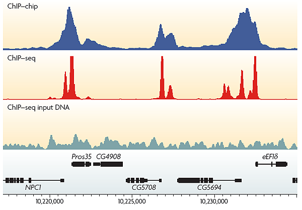
ChIP-chip與ChIP-Seq差異?
次世代定序較ChIP-chip提供更高的解析度,較少的雜訊,較少的ChIP-DNA的量,及可偵測的動態範圍及基因體範圍較廣,因此可呈現較真實的基因調控及表觀遺傳學現況。

如何分析ChIP-Seq資料?
從次世代定序儀所得到的影像檔,會轉換成核苷酸序列,並計算每個核苷酸的錯誤率,將正確性高的序列對到基因體,找到Peak後,與對照組(通常是Input DNA)比較,利用統計學的計算此Enriched region的錯誤率,之後可進行其它的分析。
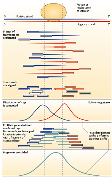
如何找到Protein binding site?
DNA是雙股的結構,因此ChIP-Seq是從DNA的5’端定序,會對到基因體的正反股,如下圖可看到藍色序列對到的是正股,紅色序列對到的是反股,因序列的數量畫出常態分佈後找到Peak,而兩者高峰處之間為Protein binding site (可稱為Enriched region)。
ChIP-Seq對照組
(1) Input DNA:免疫沉澱實驗前,取打斷的DNA當對照組,
(2) Mock IP DNA:打斷的DNA有經過免疫沈殿的實驗,但沒有加入抗體。
(3) Nonspecific IP DNA:打斷的DNA經過免疫沉澱的實驗,但有加入IgG。
這3個對照組最常用的是Input DNA,是為了矯正DNA打斷及PCR產生的bias。另外,也可以藉由Input DNA核苷酸序列的數量以及免疫沉澱後的核苷酸序列的數量之間比較,瞭解ChIP的效率,如下圖,而此圖也可以瞭解ChIP-Seq及ChIP-chip差異,前者可獲得高解析度及高敏感性的資料。
In this tutorial, we’re going to take a set of Illumina reads from an inbred Drosophila melanogaster line, and map them back to the reference genome. (After these steps, we could do things like generate a list of SNPs at which this line differs from the reference strain, or generate a genome sequence for this fly strain, but we’ll get to that later on in the course.) We are also going to use two different (but popular) mapping tools, bwa and bowtie. Among their differences is that bowtie (while smokin’ fast) does not deal with “gapped” alignments, i.e. it does not handle insertion/deletions well.
Getting the data
If you just finished the FastQC tutorial, you can keep working on the same machine. Otherwise, launch an EC2 instance, make a volume out of the same snapshot that we did before, and mount it. The data for this tutorial are in /data/drosophila:
For this example, you’ll also need the Drosophila reference genome:
%% curl -O ftp://ftp.flybase.net/genomes/Drosophila_melanogaster/dmel_r5.37_FB2011_05/fasta/dmel-all-chromosome-r5.37.fasta.gz
%% gunzip dmel-all-chromosome-r5.37.fasta.gz
Installing and running bwa
To actually do the mapping, we need to download and install bwa:
First we are going to grab the source files for bwa from sourceforge, using curl. It is important to know that we need to specify a few flags to let the program know that we want to leep the name (and filetype) for the file (-O) and that curl should follow relative hyperlinks (-L), to deal with redirection of the file site (or else curl won’t work with sourceforge).:
%% curl -O -L http://sourceforge.net/projects/bio-bwa/files/bwa-0.5.9.tar.bz2
Now we want to uncompress the tarball file using “tar”. x extracts, v is verbose (telling you what it is doing), f skips prompting for each individual file, and j tells it to unzip .bz2 files.:
%% tar xvfj bwa-0.5.9.tar.bz2
%% cd bwa-0.5.9
The make command calls a program that helps to automate the compiling process for the program.:
(Note: If your system doesn’t have make installed already, you’ll need to run “apt-get install make” before you can build bwa – but if you are using the right AMI, it should be pre-installed.)
Copy the executable for bwa to a directory for binaries which is in your shell search path:
%% cp bwa /usr/local/bin
%% cd ..
If you want to see what is in your shell search path (which can be modified later), run:
Now there are several steps involved in mapping our sequence reads and getting the output into a usable form. First we need to tell bwa to make an index of the reference genome; this will take a few minutes, so we’ve already got the index already generated in the data directory, but if you want to try it yourself, you can run (but see the note below first!!):
%% bwa index dmel-all-chromosome-r5.37.fasta
Note: This step takes several minutes. If you run it, it will overwrite the index files we have already made, so don’t run the above line exactly; instead, create a copy of the reference genome and then index the copy instead, so that we can preserve our pre-computed reference index:
%% cp dmel-all-chromosome-r5.37.fasta dmel-all-chromosome-r5.37.copy.fasta
%% bwa index dmel-all-chromosome-r5.37.copy.fasta
Next, we do the actual mapping. These were paired-end reads, which means that for each DNA fragment, we have sequence data from both ends. The sequences are therefore stored in two separate files (one for the data from each end), so we have two mapping steps to perform. For now, we’ll use bwa’s default settings. The files you’ll be running this on are datasets that have been trimmed down to just the first 1 million sequence reads to speed things up, but at the end you’ll be able to work with the final product from an analysis of the full dataset that we ran earlier (some of these steps take upwards of an hour on the full dataset, but just a couple minutes on the trimmed dataset). Run:
%% bwa aln dmel-all-chromosome-r5.37.fasta RAL357_1.fastq > RAL357_1.sai
%% bwa aln dmel-all-chromosome-r5.37.fasta RAL357_2.fastq > RAL357_2.sai
These .sai files aren’t very useful to us, so we need to convert them into SAM files. In this step, bwa takes the information from the two separate ends of each sequence and combines everything together. Here’s how you do it (this may take around 10 minutes):
%% bwa sampe dmel-all-chromosome-r5.37.fasta RAL357_1.sai RAL357_2.sai RAL357_1.fastq RAL357_2.fastq > RAL357_bwa.sam
The SAM file is technically human-readable; take a look at it with:
…It’s not very easy to understand (if you are really curious about the SAM format, there is a 12-page manual at http://samtools.sourceforge.net/SAM1.pdf). For now we’ll use bowtie to map the same reads, and we’ll use another tool to visualize these mappings in a more intuitive way.
bwa options
There are several options you can configure in bwa. Probably one of the most important is how many mismatches you will allow between a read and a potential mapping location for that location to be considered a match. The default is 4% of the read length, but you can set this to be either another proportion of the read length, or a fixed integer. For example, if you ran:
%% bwa aln -n 4 dmel-all-chromosome-r5.37.fasta RAL357_1.fastq > RAL357_1.sai
This would do almost the same thing as above, except this time, all locations in the reference genome that contain four or fewer mismatches to a given sequence read would be considered a match to that read.
Alternatively, you could do:
%% bwa aln -n 0.01 dmel-all-chromosome-r5.37.fasta RAL357_1.fastq > RAL357_1.sai
This would only allow reads to be mapped to locations at which the reference genome differs by 1% or less from a given read fragment.
If you want to speed things up, you can tell it to run the alignment on multiple threads at once (this will only work if your computer has a multi-core processor, which our Amazon image does). To do so, use the -t option to specify the number of threads. For example, the following line would run in two simultaneous threads:
%% bwa aln -t 2 dmel-all-chromosome-r5.37.fasta RAL357_1.fastq > RAL357_1.sai
bwa can also handle single-end reads. The only difference is that you would use samse instead of sampe to generate your SAM file:
%% bwa samse dmel-all-chromosome-r5.37.fasta RAL357_1.sai RAL357_1.fastq > RAL357_1.sam
Now let us align our reads using bowtie
(Note: For simplicity we are going to put all of the bowtie related files into the same directory. For your own work, you may want to organize your file structure better than we have).
Let’s get bowtie from Sourceforge:
%% curl -O -L http://sourceforge.net/projects/bowtie-bio/files/bowtie/0.12.7/bowtie-0.12.7-linux-x86_64.zip
unzip the file, and create a directory for bowtie. In this case, the program is precompiled so it comes as a binary executable:
%% unzip bowtie-0.12.7-linux-x86_64.zip
Change directory:
Copy the bowtie files to a directory in you shell search path, and then move back to the parent directory (/data/drosophila):
%% cp bowtie bowtie-build bowtie-inspect /usr/local/bin
Let’s create a new directory, “drosophila_bowtie” where we are going to place all the bowtie results:
%% cd ..
%% mkdir drosophila_bowtie
%% cd drosophila_bowtie
Now we are going to build an index of the Drosophila genome using bowtie just like we did with bwa. The original Drosophila reference genome is in the same location as we used before. Again, we have already performed the indexing step (it takes about 7 minutes), so if you want to try it yourself, index a copy so you don’t over-write the one we’ve pre-run for you:
%% bowtie-build /data/drosophila/dmel-all-chromosome-r5.37.fasta drosophila_bowtie
Now we get to map! We are going to use the default options for bowtie for the moment. Let’s go through this. there are a couple of flags that we have set, since We have paired end reads for these samples, and multiple processors. The general format for bowtie is (don’t run this):
%% bowtie indexFile fastqFile outputFile
However we have some more details we want to include, so there are a couple of flags that we have to set. -S means that we want the output in SAM format. -p 2 is for multithreading (using more than one processor). In this case we have two to use. -1 -2 tells bowtie that these are paired end reads (the .fastq), and specifies which one is which.
This should take 35-40 minutes to run on the full dataset so we’ll run it on a trimmed version (should take about 3 minutes; later we’ll give you pre-computed results for the full set.):
%% bowtie -S -p 2 drosophila_bowtie -1 /data/drosophila/RAL357_1.fastq -2 /data/drosophila/RAL357_2.fastq RAL357_bowtie.sam
You may see warning messages like:
Warning: Exhausted best-first chunk memory for read SRR018286.1830915 USI-EAS034_2_PE_FC304DDAAXX:8:21:450:1640 length=45/1 (patid 1830914); skipping read
We will talk about some options you can set to deal with this.
The bowtie manual can be found here: http://bowtie-bio.sourceforge.net/manual.shtml
Some additional useful arguments/options (at least for me) -m # Suppresses all alignments for a particular read if more than m reportable alignments exist. -v # no more than v mismatches in the entire length of the read -n -l # max number of mismatches in the high quality “seed”, which is the the first l base pairs of a read. -chunkmbs # number of mb of memory a thread is given to store path. Useful when you get warnings like above –best # make Bowtie “guarantee” that reported singleton alignments are “best” given the options –tryhard # try hard to find valid alignments, when they exit. VERY SLOW.
Viewing the output with TView
Before we can use TView to compare Bowtie and BWA mappings, we need to sort the Bowtie BAM file, and generate an index for it.:
%% cd drosophila_bowtie
%% samtools sort RAL357_full_bowtie.bam RAL357_full_bowtie.sorted
%% samtools index RAL357_full_bowtie.sorted.bam
Now that we’ve generated the files, we can view the output with TView. We’ll compare two different sorted:
%% cd ..
%% samtools tview RAL357_full_bwa.sorted.bam
Now open an additional terminal window, and load the Bowtie mapping file there as well.:
%% cd /data/drosophila/drosophila_bowtie
%% samtools tview RAL357_full_bowtie.sorted.bam ../dmel-all-chromosome-r5.37.fasta
|
|


Recent Comments