小生这厢有礼了(BioFaceBook Personal Blog)

记录生物信息学点滴足迹（NGS,Genome,Meta,Linux)

Comments Posts

英文写作检查软件汇总：人工智能帮你写论文，语法检查(转贴）

熬夜写paper的学渣小公举

如果能有一款人工智能

帮我改论文

就好了

……

没有paper，就没有伤害

我的心愿是

放飞计几，没有paper

3小时前

想太多，呵呵，别做梦了快醒醒

被paper逼疯的三更半夜，你是不是也会发出这样的感叹呢？

别着急，贴心的留学君这就来为大家介绍一些写作（检查、修改）软件：

1.StyleWriter（润色首推）

http://www.editorsoftware.com/downloads/DWSWT.html

此软件可嵌入word使用，主要功能是检查拼写、语法等错误，润色文章。会有关于同义词选择的提示，让文章的表达更加地道。Style进行文章润色的三个主要指标分别为：bog index，ave sentence, passive index。

其中，Bog index代表文章的“可读性”，其定义为 Bog Index = Sentence Bog + Word Bog – Pep

Sentencebog是句子长度决定的，等于平均句长的平方除以最大句长（long sentence limit，软件似乎设定为35个字，有点儿小气）。

而Wordbog则关乎用词，如难词、大词、专词等，也包括被动语态，这些“毛病”的总和乘以250，除以文章的总字数，最后得出的指标就是wordbog。

Peg则是一个很有趣的概念，如很好的论据和问题，有趣的表达形式等。

Bog指数包括了决定一篇文章的主要元素：单词、句子和表达形式。根据Stylewriter的标准，好文章应该是句子短小精悍，用词干净利落，而且尽量少用被动语态。反过来，句子长，词语偏，被动语态多，Bog指数就越大，文章也就越烂。好文章的bog应该在20以下。

说到这里就不能不提及，国内外有些刊物明确要求为保持文章的客观性，均不提倡在科研论文里用第一人称。但现在几乎所有讲英文写作的书，都强调多用主动语态，Stylewriter甚至说，尽可能地删除你的被动语态——虽然主动语态不等于就说we do，但很多情形是免不了的。其实，大量国际刊物都在流行we do，随便找一家刊物，在短短的几行摘要里，就能找到好几个we。因为它们本来就是“我们”做的，而不是“客观地”被做的。从这个角度来看，使用“我们”句型，不但陈述了事实，活泼了文字，也增添了科学的人文气息。

2.Triivi（检查首选）

http://www.triivi.com/

Triivi是一款功能强大的英文输入软件，基于对大量英文语料进行学习所获得的数据，Trivi具备单词、词组自动完成，拼写改错，智能学习等功能。Triivi基本词库包括接近500，000个的单词和短语，并且另外还有大量的专业词库支持，它能够帮助你提高英文输入的速度与准确度，使基于英文文本的工作更加轻松。

3.Intellicomplete(推荐)

http://www.download.com/IntelliComplete/3000-2079_4-10062169.html

Intellicomplete 是一款独特的、全功能的工具软件,使文本的处理更自动化、更高效。含有以下功能模块：自动学习并自动补足任何MS Windows应用软件中处理的单词和句子；自动扩展任何MS Windows应用软件中处理的速记以及医学缩略语;支持多个剪贴板的管理等功能。虽没有triivi专业词汇丰富，但定义性较强，且自定义语库方便，只需要一个快捷键Ctrl+Alt+J。

4.As-U-Type

http://www.asutype.com/files/asutype-setup.exe

是一款英文输入单词自动校正软件，根据软件自带的和自定义的校正词典，在编辑文档输入的单词有误时，该软件会自动提出校正意见。

但遗憾的是，As-U-Type智能在输入后按空格键后给出提示，尚不能做到实时提醒。

5.TypeTip

http://www.sharewareconnection.com/typetip.htm

与As-U-Type功能相似的辅助录入软件，而且具有实时提示及校正功能，但不能输入词组，不过兼容性较好，可作为As-U-Type以外的另一种选择。

6.金山写作助手

这是金山词霸软件的自带工具。编写英文文档时，常常会遭遇当前语境不知该用哪个单词的尴尬，这时你会怎么办？打开词霸查找一通？那太麻烦了。其实最简单的方法，是快速点击两下Alt键。这时词霸将自动弹出一个特别设计的“写作助手”模块，此时输入中文词汇，软件将自动弹出一组与搜索词对应的英文单词，如果感觉片面的解释无法帮助判断，还可以继续输入一个“分号”，这时“写作助手”将会在翻译结果中自动加入精选例句。

7.Bullfighter

www.fightthebull.com/bullfighter.asp

可用作微软Word和PowerPoint的插件，不过它只能在Windows操作系统中运行。Bullfighter的目标是找到并且删除文章中那些晦涩难懂的部分。

8.whitesomke, WriteExperss

虽然WhiteSmoke也向中国和印度的母语非英语者推销这款产品，但公司表示他们最大的目标客户群仍是那些想让自己的文笔变得典雅一些的英语母语者。

虽然在科技飞速发展的今天，依靠机器和人工智能完成文章的润色、修改甚至撰写也并非不可能，但终究无法令文字完全摆脱匠气桎梏。故而，对于Stylewriter这类神奇的文章修改软件，我们可以更多的着眼于软件标记出的“薄弱环节”，如句子冗长，用词不好，缩写不对，等等，对于这些天真而严格的批评意见，我们可以本着“有则改之无则加勉”的态度去接受。

常年在paper堆里奋战的你常用什么软件呢？

如果你有文章中没有提及的软件推荐

本文来源留学杂志，好学姐整理分享。敬请收藏哦

作者：好学姐66
链接：http://www.jianshu.com/p/d8fe428a5cdb
來源：简书
著作权归作者所有。商业转载请联系作者获得授权，非商业转载请注明出处。

Python Subprocess returns non-zero exit status only in cron

You should try to capture stderr in addition to stdout so that you can find out exactly why the program is failing (assuming it does indeed print some errors for you)


cmd = ['/path/to/casperjs', '/path/to/doSomething.js', 'args']
response = subprocess.check_output(cmd, 
                shell=True,
                stderr=subprocess.STDOUT)

0 ok    126 权限，拷贝一份，并赋予该用户所有的权限

Apache CGI Script Can Cannot Overwrite a File in a Directory it has full permissions

I ran into this due to the “SELinux” configuration. If SELinux is running, you need to explictly enable the ability for Apache to write to files. To use this, you also need to set additional permissions on those directories and files for which you are granting write access.

To determine if SELinux is enabled, execute:

sestatus

To turn on the SE booleans which enabled cgi to write to files:

sudo setsebool -P allow_httpd_anon_write 1
sudo setsebool -P allow_httpd_sys_script_anon_write 1

Then, finally to set the file/directory “SELinux security context type” to a “system” read/write file/directory (you could also make it a “public” type – Google “chcon” for info), execute this:

sudo chcon -R -t httpd_sys_rw_content_t /some/write/path

(Change /some/write/path to your path.)

BACTERIAL GENOMICS TUTORIAL （repost）

[Originally posted by Kat on her BacPathGenomics blog, April 2013]

This is a shameless plug for an article and accompanying tutorial I’ve just published together with David Edwards, my excellent MSc Bioinformatics student from the University of Melbourne. It’s currently available as a PDF pre-pub from BMC Microbial Informatics and Experimentation, but the web version will be available soon. The accompanying tutorial is available here.

The idea for this came from discussions at last year’s ASM (Australian Society of Microbiology) meeting, where it was highlighted that there was a lack of courses and tutorials available for biologists to learn the basics of genomic analysis so that they can make use of next gen sequencing. Michael Wise, a founding editor of BMC Microbial Informatics and Experimentation based at UWA in Perth, suggested the new journal would be an ideal home for such a tutorial… so here we are:

Beginner’s guide to comparative bacterial genome analysis using next-generation sequence data

http://www.microbialinformaticsj.com/content/3/1/2/

High throughput sequencing is now fast and cheap enough to be considered part of the toolbox for investigating bacteria, and there are thousands of bacterial genome sequences available for comparison in the public domain. Bacterial genome analysis is increasingly being performed by diverse groups in research, clinical and public health labs alike, who are interested in a wide array of topics related to bacterial genetics and evolution. Examples include outbreak analysis and the study of pathogenicity and antimicrobial resistance. In this beginner’s guide, we aim to provide an entry point for individuals with a biology background who want to perform their own bioinformatics analysis of bacterial genome data, to enable them to answer their own research questions. We assume readers will be familiar with genetics and the basic nature of sequence data, but do not assume any computer programming skills. The main topics covered are assembly, ordering of contigs, annotation, genome comparison and extracting common typing information. Each section includes worked examples using publicly available E. coli data and free software tools, all which can be performed on a desktop computer.

Four great tools

In the paper and tutorial, we introduce the four tools which we rely on most for basic analysis of bacterial genome assemblies: Velvet, ACT, Mauve and BRIG. All except ACT were developed as part of a PhD project, and have endured well beyond the original PhD to become well-known bioinformatics tools. New students take note!

In the paper, each tool is highlighted in its own figure, which includes some basic instructions. This is reproduced below, but is covered in much more detail in the tutorial that comes with the paper (link at the bottom).

1. Velvet for genome assembly

Possibly the most popular and widely used short read assembler, developed by the amazing Dan Zerbino during his PhD at EBI in Cambridge. Quite a PhD project!

[ Download | Paper | Protocol ]

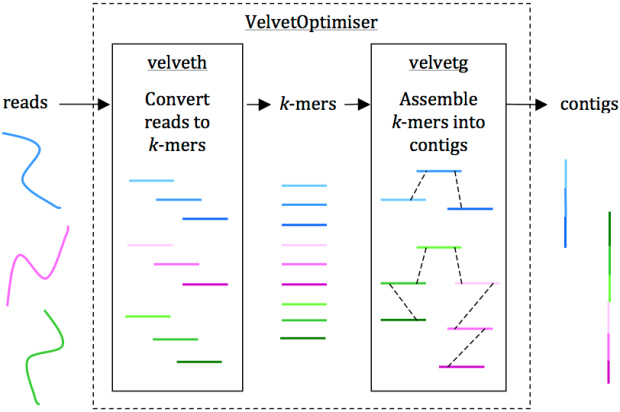
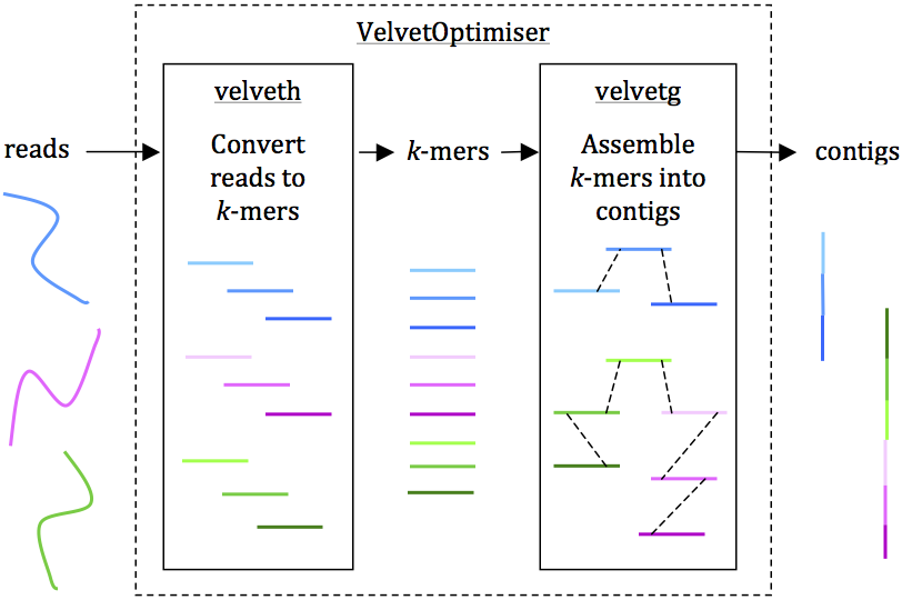
Reads are assembled into contigs using Velvet and VelvetOptimiser in two steps, (1) velveth converts reads to k-mers using a hash table, and (2) velvetg assembles overlapping k-mers into contigs via a de Bruijn graph. VelvetOptimiser can be used to automate the optimisation of parameters for velveth and velvetg and generate an optimal assembly. To generate an assembly of E. coli O104:H4 using the command-line toolVelvet:

• Download Velvet [23] (we used version 1.2.08 on Mac OS X, compiled with a maximum k-mer length of 101 bp)

• Download the paired-end Illumina reads for E. coli O104:H4 strain TY-2482 (ENA accession SRR292770)

• Convert the reads to k-mers using this command:

velveth out_data_35 35 -fastq.gz -shortPaired -separate SRR292770_1.fastq.gz SRR292770_2.fastq.gz

• Then, assemble overlapping k-mers into contigs using this command:

velvetg out_data_35 -clean yes -exp_cov 21 -cov_cutoff 2.81 -min_contig_lgth 200

This will produce a set of contigs in multifasta format for further analysis. See Additional file 1: Tutorial for further details, including help with downloading reads and using VelvetOptimiser.

2. ACT for pairwise genome comparison

Part of the Sanger Institute’s Artemis suite of tools. Also look at Artemis (single genome viewer), DNA Plotter (which can draw circular diagrams of your genomes) and BAMView (which can display mapped reads overlaid on a reference genome), they are all available here.

[ Download | Paper | Manual ]

Artemis and ACT are free, interactive genome browsers (we used ACT 11.0.0 on Mac OS X).

• Open the assembled E. coli O104:H4 contigs in Artemis and write out a single, concatenated sequence using File -> Write -> All Bases -> FASTA Format.

• Generate a comparison file between the concatenated contigs and 2 alternative reference genomes using the website WebACT.

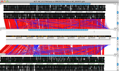
• Launch ACT and load in the reference sequences, contigs and comparison files, to get a 3-way comparison like the one shown here.

Here, the E. coli O104:H4 contigs are in the middle row, the enteroaggregative E. coli strain Ec55989 is on top and the enterohaemorrhagic E. coli strain EDL933 is below. Details of the comparison can be viewed by zooming in, to the level of genes or DNA bases.

3. Mauve for contig ordering and multiple genome comparison

Developed by the wonderful Aaron Darling during his PhD, he is now Associate Professor at University of Technology Sydney. Also see Mauve Assembly Metrics, an optional plugin for assessing assembly quality which was developed for the Assemblathon.

[ Download | Paper | User Guide ]

Mauve is a free alignment tool with an interactive browser for visualising results (we used Mauve 2.3.1 on Mac OS X).

• Launch Mauve and select File -> Align with progressiveMauve

• Click ‘Add Sequence…’ to add your genome assembly (e.g. annotated E. coli O104:H4 contigs) and other reference genomes for comparison.

• Specify a file for output, then click ‘Align…’

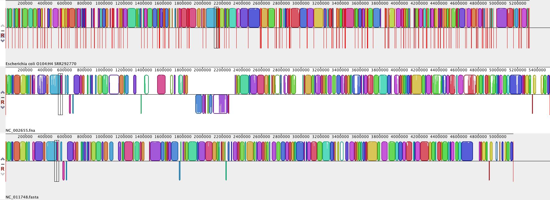
• When the alignment is finished, a visualization of the genome blocks and their homology will be displayed, as shown here. E. coli O104:H4 is on the top, red lines indicate contig boundaries within the assembly. Sequences outside coloured blocks do not have homologs in the other genomes.

4. BRIG (BLAST Ring Image Generator) for multiple genome comparison

From Nabil-Fareed Alikhan at the University of Queensland, also as part of a graduate project, which I believe is still in progress…

[ Download | Download BLAST | Paper | Tutorial ]

Fig4_BRIG

BRIG is a free tool that requires a local installation of BLAST (we used BRIG 0.95 on Mac OS X). The output is a static image.

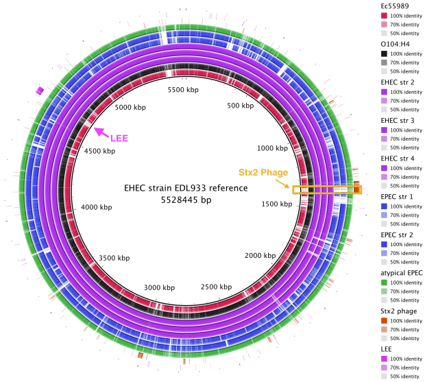
• Launch BRIG and set the reference sequence (EHEC EDL933 chromosome) and the location of other E. coli sequences for comparison. If you include reference sequences for the Stx2 phage and LEE pathogenicity island, it will be easy to see where these sequences are located.

• Click ‘Next’ and specify the sequence data and colour for each ring to be displayed in comparison to the reference.

• Click ‘Next’ and specify a title for the centre of the image and an output file, then click ‘Submit’ to run BRIG.

• BRIG will create an output file containing a circular image like the one shown here. It is easy to see that the Stx2 phage is present in the EHEC chromosomes (purple) and the outbreak genome (black), but not the EAEC or EPEC chromosomes.

Tutorial

The tutorial accompanying the article is available here. To give you an idea of what’s covered, here is the table of contents:

1. Genome assembly and annotation…………………………………………………………… 2

1.1 Downloading E. coli sequences for assembly…………………………………………….. 2

1.2 Examining quality of reads (FastQC)………………………………………………………… 2

1.3 Velvet – assembling reads into contigs………………………………………………………. 4

1.3.1 Using VelvetOptimiser to optimise de novo assembly with Velvet………….. 6

1.4 Ordering contigs against a reference using Mauve………………………………………. 7

1.4.1 Viewing the ordered contigs (Mauve)………………………………………………… 10

1.4.2 Viewing the ordered contigs (ACT)……………………………………………………. 13

1.5 Mauve Assembly Metrics – Statistical View of the Contigs………………………… 15

1.6 Annotation with RAST……………………………………………………………………………. 15

1.6.1 Alternatives to RAST………………………………………………………………………. 19

2. Comparative genome analysis……………………………………………………………….. 20

2.1 Downloading E. coli genome sequences for comparative analysis………………. 20

2.2 Mauve – for multiple genome alignment……………………………………………………. 21

2.3 ACT – for detailed pairwise genome comparisons……………………………………… 24

2.3.1 Generating comparison files for ACT…………………………………………………. 24

2.3.2 Viewing genome comparisons in ACT……………………………………………….. 27

2.4 BRIG – Visualizing reference-based comparisons of multiple sequences……… 29

3. Typing and specialist tools……………………………………………………………………. 34

3.1 PHAST – for identification of phage sequences…………………………………………. 34

3.2 ResFinder – for identification of resistance gene sequences………………………… 34

3.3 Multilocus sequence typing…………………………………………………………………….. 34

3.4 PATRIC – online genome comparison tool………………………………………………… 34

POPULATION GENOMICS OF KLEBSIELLA (Repost)

https://holtlab.net/2015/06/23/population-genomics-of-klebsiella/

Well, after almost 6 years, our Klebsiella pneumoniae genomics paper is finally out!

It’s a beast of a thing and there are still a million and one questions to address just from this one data set. For those interested in looking at the data for themselves, the raw reads are available under accessionERP000165, the assemblies are in Sylvain Brisse’s Klebsiella pneumoniae BIGSdb at the Pasteur Institute, and the tree + metadata are available for your interactive viewing pleasure in MicroReact.

The paper itself is open access in PNAS, you can read it here.

Genomic analysis of diversity, population structure, virulence, and antimicrobial resistance in Klebsiella pneumoniae, an urgent threat to public health

There have been lots of really nice Klebs genomics papers out in the last 18 months or so, examining the evolution of the ST258 clone that carries the KPC gene (K. pneumoniae carbapaenemase) and is wreaking havoc in hospitals all over the place (including recently in Melbourne), and also several hospital-based studies tracking transmission and evolution of local drug-resistant outbreaks.

But that is just the tip of the K. pneumoniae iceberg.

Our paper asks a completely different set of questions, which you could basically sum up as “what the hell is Klebsiella pneumoniae anyway?”

To do this, we sequenced ~300 genomes of really diverse K. pneumoniae strains. We didn’t have much information about genetic diversity to go on, so we chose strains with different phenotypes (antimicrobial resistance patterns, capsular serotypes or sequence types where known), from different sources (human and animal, asymptomatic carriage and infections of various kinds), and from different geographical locations.

This was done by an international group of collaborators who pooled their resources, not only sharing their precious strain collections but also digging through hospital and other records to find as much information about the strains as possible.

You can view the tree and associated metadata, including geographical origin and source information, over on Microreact. Screen Shot 2015-06-18 at 4.09.33 pm

We found out some pretty interesting things about Klebsiella pneumoniae, including the fact that what’s identified as K. pneumoniae using standard tests is actually a mixed bag of three related species, that now have their own names: K. pneumoniae (KpI group, which includes the majority of clinical isolates and all the stuff you might have heard of like the clone that causes rhinoscleromatis, and the KPC clone ST258, and the hypervirulent clone ST23); K. quasipneumoniae; and K. variicola (plant associated and usually nitrogen-fixing).

By now, this species stuff has been nutted out (mainly by co-author Sylvain Brisse from Institut Pasteur) by analysing marker gene sequences, but it’s really important to be able to show that those patterns hold at the whole-genome level, and we found some interesting things about the distribution of the rarer species (see the paper for details).

Importantly, we did the whole pan-genome analysis thing and found that as a population, K. pneumoniaehas more genes than humans. Almost 30,000 in fact. Each individual strain has ~5,500 genes, but <2,000 of those are core genes that are common to all K. pneumoniae. The rest are accessory genes that can come and go, helping the bug to adapt to new environments.

One of the cool things we were able to do with our data set, which you just can’t do with genomic studies focused on specific clones or outbreaks, was to look at statistical associations between accessory genes and phenotypes. Admittedly our available phenotypes were pretty limited, but we found a few important things.

1. VIRULENCE

We screened for genes associated with virulence in humans by focusing in on invasive infections, and comparing gene frequencies in human isolates from invasive community-acquired infections (i.e. the kind of infections that land you in hospital) vs. those in human carriage isolates or hospital acquired infections (i.e. the kind of infections that get you when you are already in hospital for something else and are particularly vulnerable to infection).

The only genes that were significantly associated with invasive infection in humans were rmpA and rmpA2, which upregulate capsule production, and genes related to iron acquisition (specifically acquired siderophore systems that can help to steal iron from animal hosts – see paper for details). These genes have been known about for some time, based on mouse models and knowledge of other pathogens, however we were able to show that these genes are significantly associated with invasive K. pneumoniaedisease in humans, which is not something that can be proven directly using experimental systems. (The siderophore story actually goes a bit deeper than the iron issue… it’s a bit too complex to go into here but I recommend reading Michael Bachman’s work e.g. “Interaction of lipocalin 2, transferrin, and siderophores determines the replicative niche of Klebsiella pneumoniae during pneumonia” in MBio, 2012).

Interestingly, doing the same test in bovine isolates showed that the story is very different: we had a lot of isolates from dairy herds, including clinical and subclinical mastitis; asymptomatic carriage isolates and strains from the farm environment… and found that an acquired lactose operon was almost perfectly associated with mastitis in cows! Something similar has been observed before in Streptococcus agalactiae.

2. ANTIBIOTIC RESISTANCE

Resistance genes were associated with human hospital isolates and human carriage isolates. This is far from an ideal study design to test this, as we had different types of collections from different geographical regions; however, even when you look within different local collections you see the same patterns: (a) comparing bovine and human isolates from NY state, the resistance genes were all in human isolates not cow isolates; (b) comparing human carriage and infection isolates (both nosocomial and community acquired) in Vietnam, the resistance genes were mainly in human carriage and hospital isolates, not in community infections; (c) in the remaining countries, isolates from infections acquired in hospital had more resistance genes than those that were considered nosocomial (diagnosed within 48 hours of admission).

What’s really interesting is that while resistance genes and virulence genes are both highly mobile components of the accessory genome, they were essentially orthogonal in their distribution. The resistance genes were mainly in hospital acquired infections and carriage isolates, whereas the virulence strains were mainly found in isolates from community acquired infections.

So far, this has resulted in the emergence of two very different kinds of K. pneumoniae clones of importance to human health: hypervirulent clones, and multidrug resistant clones. This is pretty lucky, as it means the hypervirulent clones are generally sensitive to antibiotics (although antimicrobial treatment is difficult for some conditions, like liver abscess), and the problem of untreatable highly drug resistant Klebs infections has not spread outside of hospitals.

Unfortunately, our luck appears to be runnning out and we are already starting to see the convergence of virulence and resistance. Hypervirulent ST23 strains, which have all four of the acquired siderophore systems, are accumulating antibiotic resistance genes. And about half of the KPC Klebs ST258 strains causing problems in hospitals globally have one of the siderophore gene clusters, yersiniabactin, which has been shown in clinical ST258 isolates to confer enhanced ability to cause pneumonia. How long till the other virulence genes creep in? We need to be watching!

Also, our data indicates that there are plenty of other hypervirulent or multidrug resistant Klebsclones emerging out there… convergence of virulence and resistance could happen in any one of them, so we need to be thinking and monitoring beyond the well-known ST23 and ST258 strains.

In any case, genomic surveillance is going to become really important for Klebsiella…

TOOLS FOR BACTERIAL COMPARATIVE GENOMICS

Yesterday I spoke at a workshop for JAMS TOAST (Sydney’s Joint Academic Microbiology Seminars – bioinformatics workshop)… I was asked to cover tools for comparative genomics, so I put together a list of the tried and tested programs that I find most useful for this kind of analysis. So here is the list.

First, a few caveats…

These are mostly tools with a graphical user interface (mostly Java based)… this means they should be pretty accessible to most users, however if you want to do analyses that are a bit more custom or niche, you will have to get your hands dirty and use the commandline (which you should learn to do anyway!!)

These tools are useful for small-ish scale genomic comparisons, in the order of 2-20 genomes.

Most of these tools are for assembled data, hence we start with how to assemble your data… this will become less of an issue as we move to long read sequencing with PacBio and MinION etc, but for the moment most of the data I work with is from large scale sequencing projects with Illumina (100s-1000s) so we use mapping-based approaches for a lot of tasks… so I have included a few comments about this at the end.

Beginner’s guide with walk-through tutorial

Some of these tools, particularly the visualisation of whole genome comparisons (using Artemis & ACT, Mauve, and BRIG) are covered the in the tutorial from our 2013 “Beginner’s guide to comparative bacterial genome analysis using next-generation sequence data“. So if you want a walk-through, that’s a good place to start. Please note that the links to the read sets used in the tutorial have changed, but you can still find the reads at NCBI or ENA under the accession provided (SRR292770).

First things first – Are my reads good quality?

FastQC – Generate graphical reports of read quality from the fastq files.

Assembly

SPAdes – de Bruijn graph assembly, incorporating multiple kmers and read pairing information in the building of the graph. Think of this as a more sophisticated version of Velvet… in my experience, it nearly always provides better assemblies than Velvet, except on the rare occasion (1-5% of read sets) where it fails to get a good assembly at all. In which case, try Velvet!

Velvet – The first and most widely used de Bruijn graph assembler built to tackle the problem of short reads. Graphs are built using a single kmer value, and read pairing information used for scaffolding only (unlike SPAdes, where multiple kmers are incorporated into a single graph and read pairing is also used directly in building the graph). How do you know what kmer to use? Use Velvet Optimiser. Hate the command line? Try Vague, a GUI wrapper for Velvet.

How do I judge if I have a good assembly? Try QUAST

What other assemblers are there? What’s best for what task? Take a look at Nucelotid.es and Assemblathon.

How can I view my assembly graphs? Try Bandage – freshly released from Ryan Wick, a MSc (Bioinformatics) student in my lab. Bandage allows you to view and manipulate de Druijn graphs output by Velvet or SPAdes… lots of super cool features and useful applications, see the github site for examples.

Working with assembled data

Now you have a nice set of assembled contigs – where are all the genes?

Whole genome annotation

RAST – Web tool (upload contigs), uses the subsystems in the SEED database and provides detailed annotation and pathway analysis. Takes several hours per genome but I think this is the best way to get a high quality annotation (if you have only a few genomes to annotate).

Prokka – Standalone command line tool, takes just a few minutes per genome. This is the best way to get good quality annotation in a flash, which is particularly useful if you have loads of genomes or need to annotate a pangenome or metagenome. Note however that the quality of functional information is not as good as RAST, and you will need several extra steps if you want to do functional profiling and pathway analysis of your genome(s)… which is in-built in RAST.

Annotating specific types of features

Resistance genes

CARD – best combination of easy interface + pretty good database
ARG-Annot – best quality database (in my experience, focusing on Enterobacteriaceae)
ResFinder – easy interface, database needs ongoing development

Virulence genes

PATRIC – for certain bugs only, but has good online tools for genome comparisons.
VFDB – broader range of species, but varying levels of comprehensiveness and you need to do more of the work yourself.

Insertion sequences

IS saga – Upload your genome and have IS saga find all the transposes in your genome using their IS finder database

Phage

PHAST – Upload your genome and this will identify likely prophage regions, summarising these at the level of whole phage and also individual genes.

Viewing your genome – The Artemis Genome Browser

There are zillions of genome browsers out there, but I still love Artemis… and not just because I’m from the Sanger Institute. Unlike most genome browsers, Artemis was custom-built for bacterial genomes, which let’s face it are really quite different from humans and other eukaryotes.

The default view shows you your sequence and annotation, with 6 frame translation and allows you to easily edit or create features in the annotation, graph sequence-based functions like GC content and GC skew, and do all manner of other useful things. It’s been around for a zillion years (well, at least 10 or so) and is very well developed and supported.

Artemis has lots of cool features built in, including the ‘BamView’ feature that allows you to view BAM files that show the alignment of reads mapped to your genome, zoomed in to the base level or zoomed out to look at coverage and SNP distributions… this is also super handy for viewing RNAseq data, as you can easily see the stacks of reads derived from coding regions.

Artemis also has DNA Plotter built in, which you can use to generate those pretty circular figures of your genome sequences and their features.

Plus, when you’ve got used to using Artemis to get to know your shiny new genome, you can move on toviewing comparisons against other genomes using ACT – the Artemis Comparison Tool.

Comparing whole genome assemblies

NOTE: Walk-throughs of these tools, using examples from the 2011 E. coli outbreak in Germany, are covered in the “Beginner’s guide to comparative bacterial genome analysis using next-generation sequence data“.

ACT (Artemis Comparison Tool) – Visualises BLAST (or similar) comparisons of genomes. This is most useful for comparisons of two or a few genomes, and makes it easy to spot and zoom in to regions of difference.

Mauve – Whole genome alignment and viewer that can output SNPs, regions of difference, homologous blocks, etc. It can also be used to assess assembly quality against a reference, using Mauve Contig Metrics.

BRIG (BLAST Ring Image Generator) – Gives a global view of whole genome comparisons by visualising BLAST comparisons via pretty circular figures. This is suitable for comparing lots of genomes, although because you have to enter each one through the GUI, it’s tricky to do more than a dozen or so.

Whole genome SNP-based phylogenies (from assembled data)

You can’t go past Adam Phiippy’s Harvest Suite

Parsnp – Compare genomes to a reference (using MUMmer) to identify core genome SNPs and build a phylogeny

Gingr – View the phylogeny and associated SNP calls (VCF format)… also useful for visualising tree + VCF that you have created in other ways, e.g. from mapping.

Detecting recombination in whole genome comparisons

Gubbins – A new implementation of the approach first used in Nick Croucher’s 2011 Science paper on Streptococcus pneumoniae. Command-line driven and runs pretty fast (<2 hours usually on our data).

BRAT NextGen – Uses a similar idea to Gubbins but using Bayesian clustering is GUI-driven… sounds nice, but actually I find it less convenient than Gubbins as there are manual steps required and then you need to run lots of iterations to get significance values.

Mapping based analyses

Why?

If you have specific questions to answer, where precise variant detection is important (e.g. allele calling, MLST, SNP detection, typing, mutation detection), mapping provides greater sensitivity and specificity than assembled data. Basically, if you want to be really sure about a variant call, you should be using the full information available in the reads rather than relying on the assembler and consensus base caller to get things right every time. See our SRST2 paper if you don’t believe me.

Also, if you need quick answers to specific questions, this is almost always going to be achieved faster and more accurately if you work direct from reads without attempting to generate high quality assemblies first.

The basics

For mapping our go-to is BWA or Bowtie2 (getting from fastq -> BAM). For processing of BAMs we use: SAMtools and BAMtools for variant calling, and BAMstats and BEDtools for summarising coverage and other information from the alignments.

Pipelines for specific tasks

There are loads of pipelines around the place that use the basic tools above to do specific tasks. A few of ours are:

SRST2 – MLST, resistance genes, virulence genes
ISMapper – IS (insertion sequence / tranposase) insertions
RedDog – Whole genome SNP-based phylogenies

https://holtlab.net/2015/02/25/tools-for-bacterial-comparative-genomics/

shell脚本-定时执行任务

在linux系统下，我们经常需要定时执行一些固定的任务，比如说服务器每天定时将数据进行备份，但是又不希望人工来操作，因为这样不仅效率低而且又浪费人力资源，我们可以使用shell脚本来配合crontab命令实现定时任务

centos重启命令：

reboot
shutdown -r now 立刻重启(root用户使用)
shutdown -r 10 过10分钟自动重启(root用户使用)
shutdown -r 20:35 在时间为20:35时候重启(root用户使用)

Linux centos关机命令：

halt 立刻关机
poweroff 立刻关机
shutdown -h now 立刻关机(root用户使用)
shutdown -h 10 10分钟后自动关机
如果是通过shutdown命令设置关机的话，可以用shutdown -c命令取消重启。

实现定时任务crontab

查看当前是否有定时任务

crontab -l

删除定时任务

crontab -r

每个一分钟向/CCoder/aaa.txt写入aaaaa数据

*/1 * * * * echo "aaaaa" >> /CCoder/aaa.txt

定时执行脚本

  //test.sh
   #! /bin/bash
   echo "This is Timer" >> /CCoder/aaa.txt
   exit 0

创建定时任务，注意：在执行shell脚本时必须使用绝对路径

crontab -e

编辑内容：*/1 * * * * sh /CCoder/test.sh

crontab命令介绍

基本格式：

*　 *　 *　 * 　* command　

分别表示分钟，小时，日期，月份，星期几，command表示需要执行的命令

32 20 * * * /usr/local/etc/rc.d/lighttpd restart

表示每天晚上的20:30重新启动Apache

CentOS 7通过Firewall开放防火墙端口

发现在CentOS 7上开放端口用iptables没效果(或者是sodino没找到正确的命令)…
使用firewall-cmd开放端口则立即就生效了。
见下操作：

firewall-cmd –state //查看运行状态
// 开放1024的端口
firewall-cmd –add-port=1024/tcp permanent
// 重载生效刚才的端口设置
firewall-cmd –reload

效果见下图：
firewall

firewall常用命令如下：

常用命令介绍
firewall-cmd –state ##查看防火墙状态，是否是running
firewall-cmd –reload ##重新载入配置，比如添加规则之后，需要执行此命令
firewall-cmd –get-zones ##列出支持的zone
firewall-cmd –get-services ##列出支持的服务，在列表中的服务是放行的
firewall-cmd –query-service ftp ##查看ftp服务是否支持，返回yes或者no
firewall-cmd –add-service=ftp ##临时开放ftp服务
firewall-cmd –add-service=ftp –permanent ##永久开放ftp服务
firewall-cmd –remove-service=ftp –permanent ##永久移除ftp服务
firewall-cmd –add-port=80/tcp –permanent ##永久添加80端口 
iptables -L -n ##查看规则，这个命令是和iptables的相同的
man firewall-cmd ##查看帮助

Remove grid and background from plot (ggplot2)

2013-11-27 | category RStudy | tag ggplot2

Generate data

library(ggplot2)
a <- seq(1, 20)
b <- a^0.25
df <- as.data.frame(cbind(a, b))

basic plot

myplot = ggplot(df, aes(x = a, y = b)) + geom_point()
myplot

plot of chunk ggplot-2-1

theme_bw() will get rid of the background

myplot + theme_bw()

plot of chunk ggplot-2-2

remove grid (does not remove backgroud colour and border lines)

myplot + theme(panel.grid.major = element_blank(), panel.grid.minor = element_blank())

plot of chunk ggplot-2-3

remove border lines (does not remove backgroud colour and grid lines)

myplot + theme(panel.border = element_blank())

plot of chunk ggplot-2-4

remove background (remove backgroud colour and border lines, but does not remove grid lines)

myplot + theme(panel.background = element_blank())

plot of chunk ggplot-2-5

add axis line

myplot + theme(axis.line = element_line(colour = "black"))

plot of chunk ggplot-2-6

put all together – method 1

myplot + theme(panel.grid.major = element_blank(), panel.grid.minor = element_blank(),
panel.background = element_blank(), axis.line = element_line(colour = "black"))

plot of chunk ggplot-2-8

put all together – method 2

myplot + theme_bw() + theme(panel.border = element_blank(), panel.grid.major = element_blank(),
panel.grid.minor = element_blank(), axis.line = element_line(colour = "black"))

plot of chunk ggplot-2-9

docker 删除images

docker中删除images的命令是docker rmi，但有时候执行此命令并不能删除images

[yaxin@ubox ~]$docker images
REPOSITORY          TAG                 IMAGE ID            CREATED             VIRTUAL SIZE
eg_sshd             latest              ed9c93747fe1        45 hours ago        329.8 MB
CentOS65            latest              e55a74a32125        2 days ago          360.6 MB
[yaxin@ubox ~]$docker rmi ed9c93747fe1
Untagged: ed9c93747fe16627be822ad3f7feeb8b4468200e5357877d3046aa83cc44c6af
[yaxin@ubox ~]$docker images
REPOSITORY          TAG                 IMAGE ID            CREATED             VIRTUAL SIZE
<none>              <none>              ed9c93747fe1        45 hours ago        329.8 MB
CentOS65            latest              e55a74a32125        2 days ago          360.6 MB

可以看出，image并没有被删除，只是他的tag被删除了，再次执行docker rmi IMAGE_ID只会报错

[yaxin@ubox ~]$docker rmi ed9c93747fe1
Error: image_delete: Conflict, ed9c93747fe1 wasn't deleted
2014/03/22 15:58:27 Error: failed to remove one or more images

查看docker的帮助会发现有两个与删除有关的命令rm和rmi

rm Remove one or more containers
rmi Remove one or more images

这里有两个不同的单词，images和container。其中images很好理解，跟平常使用的虚拟机的镜像一个意思，相当于一个模版，而container则是images运行时的的状态。docker对于运行过的image都保留一个状态（container），可以使用命令docker ps来查看正在运行的container，对于已经退出的container，则可以使用docker ps -a来查看。如果你退出了一个container而忘记保存其中的数据，你可以使用docker ps -a来找到对应的运行过的container使用docker commit命令将其保存为image然后运行。

回到之前的问题，由于image被某个container引用（拿来运行），如果不将这个引用的container销毁（删除），那image肯定是不能被删除。

所以想要删除运行过的images必须首先删除它的container。继续来看刚才的例子，

[yaxin@ubox ~]$docker ps -a
CONTAINER ID        IMAGE               COMMAND                CREATED             STATUS              PORTS                   NAMES
117843ade696        ed9c93747fe1        /bin/sh -c /usr/sbin   46 hours ago        Up 46 hours         0.0.0.0:49153->22/tcp   test_sshd

可以看出ed9c93747fe1的image被117843ade696的container使用着，所以必须首先删除该container

[yaxin@ubox ~]$docker rm 117843ade696
Error: container_delete: Impossible to remove a running container, please stop it first
2014/03/22 16:36:44 Error: failed to remove one or more containers

出现错误，这是因为该container正在运行中(运行docker ps查看)，先将其关闭

[yaxin@ubox ~]$docker stop 117843ade696
117843ade696

[yaxin@ubox ~]$docker rm 117843ade696
117843ade696
[yaxin@ubox ~]$docker rmi ed9c93747fe1
Deleted: ed9c93747fe16627be822ad3f7feeb8b4468200e5357877d3046aa83cc44c6af
Deleted: c8a0c19429daf73074040a14e527ad5734e70363c644f18c6815388b63eedc9b
Deleted: 95dba4c468f0e53e5f1e5d76b8581d6740aab9f59141f783f8e263ccd7cf2a8e
Deleted: c25dc743e40af6858c34375d450851bd606a70ace5d04e231a7fcc6d2ea23cc1
Deleted: 20562f5714a5ce764845119399ef75e652e23135cd5c54265ff8218b61ccbd33
Deleted: c8af1dc23af7a7aea0c25ba9b28bdee68caa8866f056e4f2aa2a5fa1bcb12693
Deleted: 38fdb2c5432e08ec6121f8dbb17e1fde17d5db4c1f149a9b702785dbf7b0f3be
Deleted: 79ca14274c80ac1df1333b89b2a41c0e0e3b91cd1b267b31bef852ceab3b2044
[yaxin@ubox ~]$docker images
REPOSITORY          TAG                 IMAGE ID            CREATED             VIRTUAL SIZE
CentOS65            latest              e55a74a32125        2 days ago          360.6 MB

可以看出，image已经被删除。

小生这厢有礼了(BioFaceBook Personal Blog)

分类

Recent Comments

链接表

英文写作检查软件汇总：人工智能帮你写论文，语法检查(转贴）

Python Subprocess returns non-zero exit status only in cron

Apache CGI Script Can Cannot Overwrite a File in a Directory it has full permissions

BACTERIAL GENOMICS TUTORIAL （repost）

Beginner’s guide to comparative bacterial genome analysis using next-generation sequence data

Four great tools

Tutorial

POPULATION GENOMICS OF KLEBSIELLA (Repost)

TOOLS FOR BACTERIAL COMPARATIVE GENOMICS

shell脚本-定时执行任务

centos重启命令：

Linux centos关机命令：

实现定时任务crontab

crontab命令介绍

CentOS 7通过Firewall开放防火墙端口

Remove grid and background from plot (ggplot2)

Remove grid and background from plot (ggplot2)

Generate data

basic plot

theme_bw() will get rid of the background

remove grid (does not remove backgroud colour and border lines)

remove border lines (does not remove backgroud colour and grid lines)

remove background (remove backgroud colour and border lines, but does not remove grid lines)

add axis line

put all together – method 1

put all together – method 2

Further reading

docker 删除images

Archives

Meta

分类

Recent Comments

链接表

Four great tools

Tutorial

centos重启命令：

Linux centos关机命令：

实现定时任务crontab

crontab命令介绍

Generate data

basic plot

theme_bw() will get rid of the background

remove grid (does not remove backgroud colour and border lines)

remove border lines (does not remove backgroud colour and grid lines)

remove background (remove backgroud colour and border lines, but does not remove grid lines)

add axis line

put all together – method 1

put all together – method 2

Further reading

Tags

Archives

Meta